A Denoising Algorithm for Quantum Remote Sensing Image Data
Bi, S. W.* Chen, H.
State Key Laboratory of Remote Sensing Science, Institute of Remote Sensing and Digital Earth, Chinese Academy of Sciences, Beijing 100101, China
Abstract: A remote sensing (RS) denoising algorithm based on the quantum-inspired concept is proposed for image denoising during RS image generation. Key benefits of the algorithm, including improvements in transmission and accuracy, were demonstrated experimentally. Firstly, the algorithm carries out a logarithmic transformation and a double density dual-tree complex wavelet transform on the noise-added image. Secondly, a denoising of the coefficients based on Bayesian theory was performed and the Maxaposterior (MAP) was used to estimate the variance of the double-tree complex wavelet. Finally, the denoised image was obtained from the inverse transform of the dual-tree complex wavelet. In comparing the final data with the original image data, we found that the peak signal to noise ratio for the proposed algorithm was improved by over 2 dB compared with classical algorithms, and the edge retention index was 0.1 higher than that for common methods.
Keywords: quantum remote sensing; image data processing; dual tree double density complex wavelet transform; Bayesian estimation; peak signal-to-noise ratio; edge-preserving index
1 Introduction
Since Professor Bi, S. W. proposed the concept “Quantum Remote Sensing (QRS)” in early 2001, the first QRS imaging prototype was developed after many stages of research, such as QRS theory, QRS information, QRS experimentation, QRS imaging, quantum spectral imaging, and QRS calculation to QRS detection[1–2]. For QRS calculations, QRS image processing methods and technologies were conducted. Based on the results of aforementioned studies, the research group of Professor Bi, S. W. has also undertaken in-depth theoretical and algorithmic experiments on QRS image processing.
Quantum image processing is a new processing method for quantum mechanics-based remote sensing (RS) images and is based on the concepts and theories of quantum mechanics, and gives full recognition to the advantages of quantum characteristics. It combines quantum mechanics theory and RS image processing technology and thus introduces a new research direction for RS image processing technology[1,3]. To date, the main achievements of this research include: a quantum denoising algorithm theory and simulation, a quantum enhancement algorithm theory and simulation, and a quantum segmentation algorithm theory research and simulation, etc. This paper focused on the first topic.
1.1 Basic Concept of QRS
The required RS image is obtained through a series of operations, including radiation and geometric correction, image embellishment, projection transformation, mosaic, feature extraction, classification, and various thematic processing steps. RS image processing can be divided into two types: optical processing, using optical, photographic and electronic methods to process RS analog images (photos, negatives); and RS digital image processing, using computers to process RS digital images to obtain the anticipated results. Conventional RS image processing methods include image embellishment processing, spatial domain processing (image grayscale enhancement), image convolution, and spatial frequency domain processing[3].
QRS is a new concept of quantum world proposed by Prof. Bi, S. W. based on traditional RS image processing methods. It reflects the motion laws of RS at the quantum level. The target for this research is the multi-space and dynamic planet-earth system with quantum mechanics as the underlying theory, and expressed by Schrodinger’s equation and the quantum states. Research was performed mainly at the technical level on QRS theory, QRS information, experimentation, imaging, calculation, measurement, calibration, quantum spectral RS and QRS application and on how to present and convey information on quantum states to our perception and reception.
QRS may help us obtain a more profound, richer and more detailed picture of information at the microscopic level. The practical aim of research on QRS is to develop a practical sensor that can be used external, whose resolution is higher than that of classical sensors[4].
1.2 Quantum Bit Representation of Images
(1) Quantum bit and quantum system
In quantum computing, a quantum state is represented by a quantum bit (or qubit), where a qubit is a two-state quantum system with two ground states. If a qubit is in two ground states expressed by  and
and  , the qubit is in a linear superposition state, which is also a possible state of the system and is represented by the following equation:
 (1)
(1)
where a and b are complex numbers that satisfy the normalization , and are called probability amplitude, and
  and
and  represent the occurrence probability of two ground states and , respectively.
If a quantum system is in the superposition of the ground states, the quantum system is coherent. When a coherent quantum system interacts with its environment in a certain way, the linear superposition will be destroyed, which is called decoherence or collapse. If a quantum system consists of n qubits, then the ith qubit state is . The state of the quantum system can be represented by the direct product of the n single qubits:
 (2)
(2)
where represents the tensor product, the state vector
  represents the ith ground state of n qubit systems
 ;
;  represents the n-bit binary number corresponding to the decimal number i;
  is the probability amplitude of the corresponding ground state; and
  is the occurrence probability of the corresponding ground state. Given that the function describes a real physical system, and that it will inevitably collapse to a ground state, the probability sum of the probability amplitude is 1 and it also satisfies the normalization condition
 .
.
(2) Pixel qubit representation
Let us assume g(m, n) is a digital image in which  ,
,  represents the pixel gray value of the image at the position of after the gray level normalization process. Clearly, g(m, n) and l-g (m, n) can be regarded as the probability of the pixel point (m, n) whose gray value is “1” and “0”, respectively. If
  and represents gray values of “0” and “1”, respectively, then the qubit of the image g(m, n) is represented as follows:
 (3)
(3)
and are introduced in the quantum system to indicate gray values of “0” and “1”, corresponding to the black and white points in the binary image. Their probability amplitudes are respectively represented as and
and when the gray values of the pixel points are “0” and “1”,
  is the qubit representations of the image g(m, n).
(3) Quantum images in quantum computers
Color image models such as RGB and HIS are needed in traditional image processing to represent colors in a standard way. In quantum computers, due to the continuity of quantum- state parameters, color can be characterized by its physical parameters (such as frequency) rather than by a linear combination of RGB, so color models are not required. Using a qubit to store color requires an instrument A to detect monochromatic electromagnetic waves and initialize the qubit according to their frequency. When different monochromatic waves are detected, they are initialized to different quantum states, where the parameter θ is proportional to the wave frequency. In this way, color information is stored in the qubit and one qubit corresponds to one pixel. To store an image, a set of quantum grids is used, which is like a matrix of qubits, represented by Q, Q={ },
},  ,
,  , that is, an image can be stored as a quantum grid. The set of quantum grids R is represented by
  ,
,  , therefore,
  , containing
  qubits[5–8].
1.3 Quantum Image Data Processing
Quantum image data processing: Assuming that the input data (the image) is stored in electronic memory, correspondingly, the quantum state preparation means that the image information is implicit in the quantum state. Based on image processing methods, unitary transformation is applied to the quantum state and then the quantum state is detected to obtain the solution. This process is called quantum image processing.
1.4 QRS Image Processing
QRS image processing includes two types. One is based on traditional RS data and traditional computing, which is called primary QRS image processing in this paper; the second one is based on QRS and quantum computing, which is called advanced QRS image processing in this paper[3].
(1) Primary QRS image processing
This method draws on and uses the basic concepts and principles of quantum mechanics, and takes advantages of quantum characteristics. It is a new or improved method of RS image processing based on the principles of quantum mechanics by using traditional computors. This method does not rely on quantum-level physical equipment, but instead involves the organic combination of quantum mechanics theory and RS image processing technology, introducing a new theoretical tool for RS image processing technology.
(2) Advanced QRS image data processing
In accord with the laws of quantum mechanics, this approach aims to study image data based on quantum optics and quantum information theory, taking quantum state as the information carrier to reflect the motion laws of imaging at the quantum level. This method can fundamentally improve the image resolution and image quality. It aims to store QRS information and perform QRS calculations by using quantum computing. The approach adopts quantum algorithms, whose calculation speed has increased exponentially compared with conventional algorithms, providing a new way to solve the RS image data processing speed issue which is currently not fast enough.
The steps of advanced QRS image processing methods are as follows: 1) Processing images via quantum mechanics (using quantum states) requires a device to convert frequencies into quantum states, and then quantum bit lattices are used to store images for quantum image extraction; 2) Processing images with entangled quantum systems (using quantum bit states) to store the structure and content of simple images in a quantum system. Advanced QRS image data processing technology requires many technologies and methods such as software, data processing devices, and image data processing techniques.
2 Introduction to Quantum Denoising Algorithm
2.1 Research Background
Classical image denoising methods mainly include two kinds: spatial domain and transform domain. Classical methods in the spatial domain, which include adaptive median filtering[9], Lee filtering[10] and Frost filtering[11], can eliminate noises to a certain extent, but the processed images are poor edge-preserved and blurred[12]. The spatial domain mainly include frequency and wavelet transforms. As wavelet transform inherent multi-frequency analysis and good local time and frequency domain characteristics, it shows outstanding advantages for synthetic aperture redar (SAR) image denoising processing[13–14]. Pizurica et al. proposed a wavelet domain medical image denoising method using Bayesian theory, but still with limited denoising and edge retention ability[15]. Khare et al. proposed a denoising method based on complex wavelet transform, which used the imaginary product of adjacent scale complex wavelet coefficients to detect strong edges, and then shrink the wavelet coefficients of non-strong edges in the wavelet domain, thus achieving some denoising effect[16]. Sendur et al. proposed a method based on a nonlinear bi-variate contraction function (BI-DTCWT), which is simple and effective for additive noise filtering. Combined with logarithmic transformation, the BI-DTCWT method is effective in filtering speckle noise[17]. The double density dual-tree complex wavelet transform combines the advantages of dual-tree complex transforms and double density complex wavelet transform, making it more advantageous in image processing such as image segmentation, speckle reduction and enhancement[10–12].
2.2 Quantum Superposition State
In quantum computing, information is encoded by and states to quantify classical information. Inspired by quantum superposition theory, we use and states to represent the noise state and signal state respectively, and then encode the wavelet coefficients[17]. The signal wavelet coefficients between scales have a strong correlation with the noise level. In the image speckle method proposed in this paper, the product expression of the parent-progeny wavelet coefficient is:
 (4)
(4)
where θ can take six directions, ±15°, ±45° and ±75°;  represents the product of the parent coefficient modulus
  in the position (i, j) and the current progeny coefficient modulus
  in the sub-band image in scale s direction θ. According to the quantum superposition state principle, the product of the high-frequency sub-band parental-progeny wavelet coefficient can be considered as the superposition of the two quantum states of noise and signal:
  , where a and b represent the probability amplitude of the quantum ground state and state, respectively.
  and indicate the measurement probability of the noise stateand the signal state
  , respectively, and the normalization condition must be satisfied. In the high frequency sub-band, the signal corresponds to the edge and detail of the image. Assuming
  is normalized ,
  . In the algorithm proposed in this paper,
  is defined as:
 (5)
(5)
where  and
and  represent the occurrence probability of signal and noise, respectively, of the wavelet-derived quantum-derived at position (i, j) in the wavelet sub-band in scale s direction θ.
2.3 Double Density Dual-tree Complex Wavelet Transform
The double density dual-tree complex wavelet transform (DD-DTCWT) uses three Hilbert filter pairs where  is the low-pass filter,
  is the first-order high-pass filter and
  the second- order high-pass filter, and the two-dimensional double density dual-tree complex wavelet transform has two scales and four resolution functions, that is,
 ,
, , i=1, 2.
Two wavelet functions are obtained by offsetting half of another function, that is,
 (6)
(6)
An approximate Hilbert transform pair is formed between the two sets of wavelet functions,
 . (7)
. (7)
The DD-DTCWT can be realized by two sets of three pairs of filters acting on the input data at the same time. Each layer of the DD-DTCWT not only decomposes the low frequency part but also further decomposes the two high-pass filters; meanwhile the iterative filter bank of the upper tree A represents the real part of the complex wavelet transform, and the iterative filter bank of the lower tree B represents the imaginary part of the complex wavelet transform, forming a double density dual-tree complex wavelet transform[19,21] (Figure 1), that is,
 (8)
(8)
Figure 1 Flow chart of two-dimensional double density dual-tree complex wavelet transform
2.4 Algorithm Steps
The algorithm was conducted in the following steps:
Step 1: carry out a logarithmic transform of the SAR image, convert the multiplicative speckle noise in the image into additive noise, and decompose the transformed image into a double density dual-tree complex wavelet.
Step 2: After that, the wavelet coefficients of each layer are obtained, with high-frequency, low-frequency components and angle information, then normalize the data.
Step 3: According to Bayesian theory, use the Bayesian Maxaposteriori Estimation (MAP):
 (9)
(9)
Deriving the wavelet coefficient x, we can get
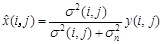 (10)
(10)
The above equation shows that after calculating the standard deviation  of the signal and the standard deviation of the noise, the value of the wavelet coefficient x can be obtained.
Step 4: Introduce the quantum derivative formula:
 (11)
(11)
The noise variance equation is:
 (12)
(12)
where  represents the real part of the wavelet high frequency subband coefficient in the 45° direction, and the signal variance equation is:
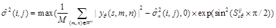 (13)
(13)
Step 5: Introduce the quantum derivative denoising factor into equation (8), calculate the wavelet coefficient x, and perform the DD-DTCWT inverse transformation.
Step 6: Perform exponential transformation on the coefficients of each column and each row to obtain the denoised image.
2.5 Evaluation Functions
The mean square error (MSE) function is:
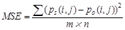 (14)
(14)
The peak signal to noise ratio (PSNR) function is:
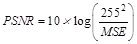 (15)
(15)
The edge preserving index (EPI) function is:
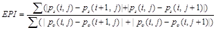 (16)
(16)
where m × n is the pixel value of the processed image, and  is the gray value of the resulting image in the ith row and the jth column . Similarly,
  is the gray value of the original noise image pixel at the same position, and and are in the edge area. The minimum EPI is 0 and the maximum is 1[22–23].
3 Denoising Algorithm Flow for Quantum Image Data
|
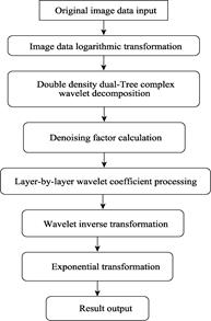
Figure 2 Quantum image data denoising algorithm flow chart
|
The denoising algorithm flow is shown in Figure 2. The main steps include: input of original image data, logarithmic transformation of image data, double density dual-tree complex wavelet decomposition, denoising factor calculation, layer-by-layer wavelet coefficient processing, wavelet inverse transformation, exponential transformation, and result output.
4 Quantum Image Data Denoising Algorithm Simulation Experiment and Results
Two separate sets of experiments were conducted with the same three parameters, namely, the addition of uniform random noise with (1) mean value of 0 and variance of 0.04; (2) mean value of 0 with variance of 0.1; (3) mean value of 0 with variance of 0.3.
4.1 Results for the First Set of Experiments
4.1.1 Uniform Random Noise with Mean Value of 0 and Variance of 0.04
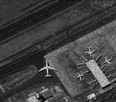
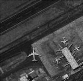
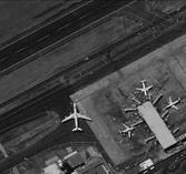
Figure 3 shows the denoising results for the quantum algorithm, the Frost algorithm, the Median filtering, and the Wiener algorithm after the addition of noise (mean value of 0, variance of 0.04) compared with the original image and the noise-added image. Table 1 lists the evaluation parameters for noise reduction. Among them, the PSNR and the EPI of the quantum algorithm was higher than that of the other algorithms (Table 1), indicating that the quantum algorithm performed the best. Also the PSNR of the quantum algorithm was 9.41% higher than the other algorithms. Furthermore, the EPI of the quantum algorithm was 60.38% higher than the three traditional algorithms (Table 1, Figure 3). Among them, Improvement percentage=(results of Quantum algorithm-results of the other algorithms)/results of the other algorithms (the same below).
4.1.2 Uniform Random Noise with Mean Value of 0 and Variance of 0.1
Figure 4 shows the denoising results for different algorithms after addition of noise (mean value of 0, variance of 0.1) compared with the original image and the noise-added image and Table 2 lists the noise reduction evaluation parameters. Among them, the PSNR and the EPI of the quantum algorithm was higher than that of the other algorithms (Table 2), indicating that the quantum algorithm performed the best. Also the PSNR of the quantum algorithm was 10.89% higher than the three traditional algorithms, and the EPI for the quantum algorithm was 50% higher than the three traditional algorithms (Table 2, Figure 4).
4.1.3 Uniform Random Noise with Mean Value of 0 and Variance of 0.3
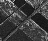
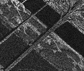
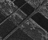
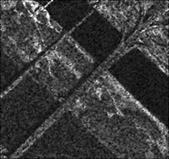
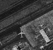
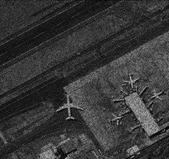
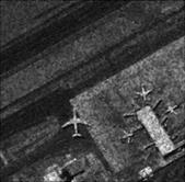
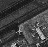
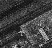
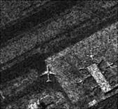
Figure 5 shows the denoising results for different algorithms after the addition of uniform random noise with a mean value of 0 and a variance of 0.3 compared with the original image and the noise-added image. Table 3 lists the noise reduction evaluation parameters. Among them, the PSNR and the EPI of the quantum algorithm were higher than those of the other algorithms (Table 3), indicating that the quantum algorithm gave the best performance. Also the PSNR for the quantum algorithm was 14.54% higher than the three traditional algorithms, and the EPI for the quantum algorithm was 38.6% higher than the three traditional algorithms (Table 3, Figure 5).


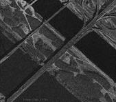
(a) Original image (b) Noise-added image. (c) Quantum algorithm
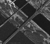
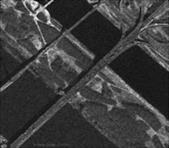

(d) Frost (e) Median filtering (f) Wiener
Figure 3 Experimental results for uniform random noise with mean value of 0 and variance of 0.04.
Table 1 Comparison of the denoising results for the different processing methods after addition of noise (mean value of 0, variance of 0.04)
|
Processing method
|
PSNR
|
Improvement percentage (%)
|
EPI
|
Improvement percentage (%)
|
|
Quantum algorithm
|
25.344,7
|
-
|
0.85
|
-
|
|
Frost
|
21.326,7
|
18.84
|
0.53
|
60.38
|
|
Median filtering
|
22.538,7
|
12.45
|
0.36
|
136.11
|
|
Wiener
|
23.165,9
|
9.41
|
0.52
|
63.46
|
4.2 Results for the Second Set of Experiments
4.2.1 Uniform Random Noise with Mean Value of 0 and Variance of 0.04
Figure 6 shows the denoising results for different algorithms after the addition of uniform random noise (mean value of 0, variance of 0.04) compared with the original image and the noise-added image and Table 4 lists the noise reduction evaluation parameters. Among them, the PSNR and the EPI of the quantum algorithm were higher than those of the other algorithms (Table 4), indicating that the quantum algorithm gave the best performance. Also the PSNR for the quantum algorithm was 13.83% higher than the three traditional algorithms. Further, the EPI for the quantum algorithm was 75% higher t han the three traditional algorithms (Table 4, Figure 6).


(a) Original image (b) Noise-added image (c) Quantum algorithm


(d) Frost (e) Median filtering (f) Wiener
Figure 4 Experiment results for uniform random noise with mean value of 0 and variance of 0.1
Table 2 Comparison of denoising results for the different processing methods after addition of uniform random noise with mean value of 0 and variance of 0.1
|
Processing method
|
PSNR
|
Improvement percentage
(%)
|
EPI
|
Improvement percentage
(%)
|
|
Quantum algorithm
|
25.35
|
-
|
0.84
|
-
|
|
Frost
|
18.48
|
37.18
|
0.56
|
50.00
|
|
Median filtering
|
19.76
|
28.29
|
0.32
|
162.50
|
|
Wiener
|
22.86
|
10.89
|
0.45
|
86.67
|
4.2.2 Uniform Random Noise with Mean Value of 0 and Variance of 0.1
Figure 7 shows the denoising results for different algorithms after addition of uniform random noise (mean value of 0, variance of 0.1) compared with the original image and the noise-added image.

(a) Original image (b) Noise-added image (c) Quantum algorithm


(d) Frost (e) Median filtering (f) Wiener
Figure 5 Experimental results for uniform random noise with mean value of 0 and variance of 0.3
Table 3 Comparison of denoising results for the different processing methods after addition of uniform random noise with mean value of 0 and variance of 0.3
|
Processing method
|
PSNR
|
Improvement percentage (%)
|
EPI
|
Improvement percentage (%)
|
|
Quantum algorithm
|
22.30
|
-
|
0.79
|
-
|
|
Frost
|
14.87
|
49.97
|
0.57
|
38.60
|
|
Median filtering
|
15.98
|
39.55
|
0.33
|
139.39
|
|
Wiener
|
19.47
|
14.54
|
0.41
|
92.68
|


(a) Original image (b) Noise-added image (c) Quantum algorithm


(d) Frost (e) Median filtering (f) Wiener
Figure 6 Experimental results for uniform random noise with mean value of 0 and variance of 0.04
Table 5 lists the evaluation parameters for noise reduction. Among them, the PSNR and the EPI of the quantum algorithm were higher than those of the other algorithms (Table 5), indicating that the quantum algorithm performed the best. Also the PSNR for the quantum algorithm was 11.01% higher than the three traditional algorithms. Furthermore, the EPI for the quantum algorithm was 58.18% higher than that of the three traditional algorithms (Table 5, Figure 7).
Table 4 Comparison of denoising results for the different processing methods after addition of uniform random noise with mean value of 0 and variance of 0.04
|
Processing method
|
PSNR
|
Improvement percentage (%)
|
EPI
|
Improvement percentage (%)
|
|
Quantum algorithm
|
25.43
|
-
|
0.91
|
-
|
|
Frost
|
20.84
|
22.02
|
0.52
|
75.00
|
|
Median filtering
|
21.98
|
15.70
|
0.31
|
193.55
|
|
Wiener
|
22.34
|
13.83
|
0.44
|
106.82
|
(a) Original image (b) Noise-added image (c) Quantum algorithm

(d) Frost (e) Median filtering (f) Wiener
Figure 7 Experimental results for uniform random noise with mean value of 0 and variance of 0.1
Table 5 Comparison of denoising results for the different processing methods after addition of uniform random noise with mean value of 0 and variance of 0.1
|
Processing method
|
PSNR
|
Improvement percentage (%)
|
EPI
|
Improvement percentage (%)
|
|
Quantum algorithm
|
24.40
|
-
|
0.87
|
-
|
|
Frost
|
18.14
|
34.51
|
0.55
|
58.18
|
|
Median filtering
|
19.38
|
25.90
|
0.47
|
85.11
|
|
Wiener
|
21.98
|
11.01
|
0.40
|
117.50
|
4.2.3 Uniform Random Noise with Mean Value of 0 and Variance of 0.3
Figure 8 shows the denoising results for different algorithms after addition of uniform random noise (mean value of 0, variance of 0.3) compared with the original image and the noise-added image. Table 6 lists the noise reduction evaluation parameters. Among them, the PSNR and the EPI of the quantum algorithm were higher than those of the other algorithms (Table 6), indicating that the quantum algorithm gave the best performance. Also, the PSNR of the quantum algorithm was 18.83% higher than that of the three traditional algorithms. Furthermore, the EPI of the quantum algorithm was 42.86% higher than that of the three traditional algorithms (Table 6, Figure 8).


(a) Original image (b) Noise-added image (c) Quantum algorithm


(d) Frost (e) Median filtering (f) Wiener
Figure 8 Experimental results for uniform random noise with mean value of 0 and variance of 0.3
Table 6 Comparison of denoising results for different processing methods after the addition of uniform random noise with mean value of 0 and variance of 0.3
|
Processing method
|
PSNR
|
Improvement percentage (%)
|
EPI
|
Improvement percentage (%)
|
|
Quantum algorithm
|
22.34
|
-
|
0.80
|
-
|
|
Frost
|
14.60
|
53.01
|
0.56
|
42.86
|
|
Median filtering
|
15.71
|
42.20
|
0.32
|
150.00
|
|
Wiener
|
18.80
|
18.83
|
0.38
|
110.53
|
4.3 Summary of Two Sets of Experiments
From the results of the two sets of experiments, it is clear that both the PSNR and the EPI of the quantum algorithm were higher than those of the three conventional algorithms. Specifically, (1) for the addition of noise with mean value of 0 and variance of 0.04, the PSNR and the EPI of the quantum denoising algorithm were 10%-20% and 60%-160% higher than those of the classical algorithms, respectively (Table 7); (2) for the addition of noise with mean value of 0 and variance of 0.1, the PSNR and EPI of the quantum denoising algorithm were 10%-35% and 50%-120% higher than those of the classical algorithms, respectively (Table 8); and (3) for the addition of noise with mean value of 0 and variance of 0.3, the PSNR and EPI of the quantum denoising algorithm were 15%-50% and 40%-140% higher than those of the classical algorithms, respectively (Table 9).
5 Discussion and Conclusion
The two sets of experiments demonstrated that the quantum denoising algorithm performed better than the three conventional algorithms. The PSNR obtained by the quantum algorithm was 2 dB higher than that afforded by conventional methods, and the EPI was higher by more than 0.1 relative to the common methods. The quantum denoising method performed well in recovery of contour information, effectively being able to distinguish image signals from noise, enhancing the adaptability of local filtering, and preserving more image edge details. Therefore, the performance of the quantum denoising algorithm was significantly improved compared to the conventional methods.
The proposed algorithm combines the DD-DTCWT, Bayesian theory, and quantum derivative thought and achieves good experimental results. Combining the DD-DTCWT with quantum derivative methods can promote each other, and better address the contradiction between on the one hand denoising smoothing and maintaining detail, and on the other hand improving the image processing quality. Experimental results showed that the quantum image denoising algorithm performed very well in image detail retention and presented enhanced visual effects and data precision.
Table 7 Average improvement percentage of quantum processing method than other algorithms in two denoising experiments with noise whose mean value being 0 and variance being 0.04
|
Processing method
|
PSNR
|
EPI
|
|
Frost
|
20.43%
|
67.69%
|
|
Median filtering
|
14.08%
|
164.83%
|
|
Wiener
|
11.62%
|
85.14%
|
Table 8 Average improvement percentage of quantum processing method than other algorithm in two denoising experiments with noise whose mean value being 0 and variance being 0.1
|
Processing method
|
PSNR
|
EPI
|
|
Frost
|
35.85%
|
54.09%
|
|
Median filtering
|
27.10%
|
123.81%
|
|
Wiener
|
10.95%
|
102.09%
|
Table 9 Average improvement percentage of quantum processing method than other algorithm in two denoising experiments with noise whose mean value being 0 and variance being 0.3
|
Processing method
|
PSNR
|
EPI
|
|
Frost
|
51.49%
|
40.73%
|
|
Median filtering
|
40.88%
|
144.70%
|
|
Wiener
|
16.69%
|
101.61%
|
The past two years have witnessed an acceleration in research and development in the quantum computing and quantum communication fields, while progress in quantum image processing has been modest, despite efforts by the team of Professor Bi to address the latter. Given that quantum computers have not yet been developed, and current photon quantum computing prototypes cannot realize general-purpose computing but can only be used for Bose sampling, the capacity of existing photon quantum computing prototypes is restrained in some specific tasks, making it especially important to develop quantum image processing at this early stage. When quantum computers become available, the quantum image processing theory and technology could be developed more efficiently.
References
[1] Bi, S. W. Research on the concept, framework and connotation of quantum remote sensing [J]. Journal of Infrared and Millimeter Waves, 2003, 22(Sup.): 1-9.
[2] Bi, S. W., Han J. X. The mid-far infrared experiment of quantum remote sensing [C]. Beijing: Proceedings of the 15th National Remote Sensing Conference, 2005: 8-15.
[3] Tang, G. A., Zhang, S. Y., Liu, Y. M., et al. Processing of remote sensing image data [M]. Beijing: Science Press, 2004.
[4] Bi, S. W., Han J. X. Research on quantum remote sensing information mechanism [J]. Science & Technology Review, 2006, 9(11): 38-42.
[5] Fu, X. W., Dai, W., Chen, L. Despeckle of ultrasound-derived ultrasound images based on local entropy [J]. Journal of Electronics & Information Technology, 2015, 37(3): 560-566.
[6] Xie, K. F. Research on quantum derivative image processing method [D]. Changsha: Central South University, 2007: 1-119.
[7] Xie, K. F, Luo, A., Zhou, X. Y. Edge detection method of quantum derived morphology [J]. Computer Engineering and Applications, 2007, 43(11): 87-90.
[8] Zhang, Y. Research on remote sensing image processing based on quantum derivation [D]. Beijing: University of Chinese Academy of Sciences, 2015: 1-67.
[9] Jiang, Y., Zhang, X. L., Shi, J. Improved Lee filtering speckle reduction for polarized SAR [J]]. Journal of University of Electronic Science and Technology of China. 2009, 38(1): 5-8.
[10] Zhang, X. M., Xu, B. S., Dong, S. Y. Adaptive median filtering for image processing [J] Journal of Computer- Aided Design & Computer Graphics, 2005, 17: 295-299.
[11] Zhang, Z. H., Pan, C. H., Ma, Y. D. A speckle noise reduction method for SAR images based on modified frost kernel [J]. Journal of Image and Graphics, 2005, 10(4): 431-435.
[12] Liu, L. J., Hu, S. Y., Cao, X. H. Study on speckle noise suppression of SAR image based on Q-Shift dual- tree complex wavelet [J]. Tactical Missile Technology, 2014(4): 82-86.
[13] Chen, L. N., Tang, Z., Gao, Z., et al. A SAR Image denoising method based on wavelet threshold [J]. Ocean Surveying and Mapping, 2009, 29(5): 48-50.
[14] Liu, C. X. Research on image denoising algorithm of mobile phone camera based on wavelet transform [D]. Chongqing: Southeast University, 2016.
[15] Pizurica, A., Philips, W., Lemahieu, I., et al. A versatile wavelet domain noise filtration technique for medical imaging [J]. IEEE Trans Med Imaging, 2003, 22(3): 323-331.
[16] Khare, A., Khare, M., Jeong, Y., et al. Despeckling of medical ultrasound images using daubechies complex wavelet transform [J]. Signal Process, 2010, 90(2): 428-439.
[17] Sendur, L., Selesnick, I. W. Bivariate shrinkage functions for wavelet based denoising exploiting interscale dependency [J]. IEEE Trans Signal Process, 2002, 50(11): 2744-2756.
[18] Kingsbury, N. G. The dual-tree complex wavelet transform: a new technique for shift invariance and directional filters [C]. Proc IEEE Dsp Workshop, 1998: 319-322
[19] Selesnick, I. W., Baraniuk, R. G., Kingsbury, N. G. The dual-tree complex wavelet transform [J]. IEEE Signal Processing Magazine, 2005, 22(6): 123-151.
[20] Guo, W., Zhang, P. Research on image denoising of synthetic aperture radar based on double density dual- tree complex wavelet transform [J]. Acta Electronica Sinica, 2009, 37(12): 2747-2752
[21] Du, Y. F., Wang, J. J. Seismic signal denoising of double density dual-tree complex wavelet domain statistical model [J]. Journal of Hefei University of Technology: Natural Science Edition, 2018, 41(7): 995-1001.
[22] Chen, R. Y., Zhang, F. Y., Shi, L. W. Image quality assessment based on human visual model and singular value decomposition in Contourlet domain [J]. Journal of Optoelectronics·Laser, 2010, 21(10): 1560-1560.
[23] Zhang, W., Sun, R. H., Zhang, X. C. Noised removal of SAR image based on improved wavelet soft thresholding method [J]. Remote Sensing Information, 2004(4): 4-6.