Global Land Slope Frequency Dataset
Tang, L.1
Ma, J. W.1 Shao,
Z. Y.1 Peng, Q. Z.1,2*
1. Faculty of Land Resources Engineering, Kunming
University of Science and Technology, Kunming 650093, China;
2. Surveying and Mapping Geo-Informatics
Technology Research Center on Plateau Mountains of Yunnan Higher Education,
Kunming 650093, China
Abstract: Slope frequency distribution can quantitatively measure slope,
which is an important factor in landform characterization. The absence of
high-resolution global slope frequency distribution hinders cross-regional
comparative analysis. Obtaining 30 m digital elevation models (DEMs) covering a
large land area??ASTER GDEM v3.0??permits quantitative slope analysis of Earth??s
surface at an unprecedented scale and resolution. We used the ArcGIS Slope and Int routine to obtain the integer slope data in 90 intervals and
then calculated the slope frequency distribution for 3 statistic units: 1??
(latitude) ??1?? (longitude) grids, the 7 continents, and the globe. These areas
are different in scale, climate, and tectonic history, but their slope
distributions are consistently unimodal. The peak in each distribution appears
before 5??. 50% of the total ground surface has a slope less than 5.5??, the land
surface slope of Oceania is the most gentle (?? = 5.23??) with the most concentrated distribution (?? = 5.31??), and the ice sheet surface
slope of Antarctica is the steepest (??
= 13.53??) with the most dispersed distribution (?? = 15.86??). The data include the land slope frequency
distributions for 3 statistic units, 1?? (latitude) ??1?? (longitude) grid with 22,205
data records in total, 7 continents, and the Earth in .xlsx format and the land
slope frequency spatial distribution for the 1??x1?? grids in .shp format. The
dataset is archived in 631 data files, with a size of 232 MB (compressed to
54.5 MB in one file).
Keywords: globe; land; slope
frequency distribution; ASTER GDEM grid
1 Introduction
The slope frequency distribution is the proportion of the
total surface falling within certain slope classes, into which the total
angular range of slope is subdivided[1]. The slope frequency
distribution is a powerful tool for describing topography and has been
successfully employed for analysis of planetary landforms[2‒5],
geologic hazards[6‒7], and regional landscapes and geomorphology[8‒9].
A slope frequency distribution can provide regional landform characteristics
(e.g. the dominant slope angle) but is not easily comparable across regions.
Hence, early studies focused on the identification of transformations of slope
data to normalized slope distributions[10‒11]. Subsequent studies
attempted to relate slope frequency distributions to landscape patterns[12?C14];
however, regional slope analysis can only provide a reference for a single
region because regional slope-frequency distributions show vastly different
characteristics. Thus, it is necessary to establish a global benchmark for
slope frequency distributions so that different studies can be compared.
The slope is a scale-dependent parameter that changes
with the digital elevation model (DEM) resolution. As such slope is not
comparable between DEMs with different resolutions[15]. The first
global land slope frequency distribution appeared in 1985 with a spatial resolution
of 1??[2] and has been used to compare the global topographic
characteristics of Venus and Earth. Subsequently, the prevalent resolution of
global DEM data, which is easy to obtain, has been refined to 1?? (about 30
m); however, no study has calculated a global slope distribution using 30 m DEM
data. In this contribution, the ASTER GDEM v3.0 DEM which nearly covers Earth??s
entire land surface at 30 m resolution[16], was used to calculate
the slope angle and generate a global land slope histogram, which can provide a
reference for cross-regional slope analysis.
2 Metadata of the Dataset
The
metadata of the ??Global land slope frequency dataset??[17] is
summarized in Table 1. It includes the dataset full name, short name, authors,
spatial resolution, data format, data size, data files, data publisher, and
data sharing policy, etc.
Table 1 Metadata summary of ??Global land slope
frequency dataset??
|
Items
|
Description
|
|
Dataset
full name
|
Global land slope frequency dataset
|
|
Dataset
short name
|
LSF_Globe
|
|
Authors
|
Tang,
L. D-4700-2019, Faculty of Land Resources Engineering,
Kunming University of Science and Technology, 799643248@qq.com
Ma,
J. W. AAG-3726-2019, Faculty of Land
Resources Engineering, Kunming University of Science and Technology, 359424547@qq.com
Shao,
Z. Y. AAG-3633-2019, Faculty of Land
Resources Engineering, Kunming University of Science and Technology, 785383110@qq.com
Peng, Q. Z. AAG-3629-2019, Faculty of Land
Resources Engineering, Kunming University of Science and Technology, pqz20002@163.com
|
|
Geographical
region
|
The
land surface from 83??N to 83??S
|
|
Data
format
|
.xlsx,
.shp Data
size 54.5 MB (after compression)
|
|
Data
files
|
1??(latitude)´1??(longitude)
grid land slope frequency distribution, 7 continents, and global land slope
frequency distributions
|
|
Foundation
|
National
Natural Science Foundation of China (41961039)
|
|
Computing
environment
|
ArcGIS
10.2 (shared within the departmental research group)
|
|
Data
publisher
|
Global Change Research Data Publishing &
Repository, http://www.geodoi.ac.cn
|
|
Address
|
No.
11A, Datun Road, Chaoyang District, Beijing 100101, China
|
|
Data
sharing policy
|
Data from
the Global Change Research Data Publishing & Repository includes metadata,
datasets (data products), and publications (in this case, in the Journal of Global Change Data & Discovery). Data sharing policy include: (1) Data
are openly available and can be freely downloaded via the Internet; (2) End
users are encouraged to use Data subject to citation; (3)
Users, who are by definition also value-added service providers, are welcome
to redistribute Data subject to written permission from the GCdataPR Editorial
Office and the issuance of a Data redistribution license; and (4) If Data
are used to compile new datasets, the ??ten percent principal?? should be
followed such that Data records utilized should not
surpass 10% of the new dataset contents, while sources should be noted in
suitable places in the new dataset[18]
|
|
Communication
and
searchable
system
|
DOI,
DCI, CSCD, WDS/ISC, GEOSS, China GEOSS, Crossref
|
3 Methods
Slope data for slope frequency distribution analysis
were computed using the 30 m ASTER GDEM v3.0 (GDEM v3)[19], which
provides land surface coverage of Earth from 83??N to 83??S latitude with 22,912
tiles. The elevation value of the ocean is 0 m which will influence the
frequency value at 0?? slope; hence, we use the 1:1,000,000 global base map data
as a mask to remove the oceans from the GDEM v3. The global land slope
frequency distribution dataset can be divided into three categories: 1?? (latitude)
?? 1?? (longitude) grid land slope frequency, 7 continents land slope frequency,
and global land slope frequency.
The acquisition of slope frequency distribution data primarily required
two steps: slope calculation and slope frequency calculation. Because the DEM
dataset has 22,912 scenes in total, the scene by scene calculation takes a long
time and is prone to errors; hence, a Python (v2.7.0) script was compiled to
automate the calculation process.
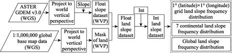
Figure 1
Flowchart
of the dataset processing
The projected
coordinate system used in this study is the world vertical perspective (WVP),
which has a vertical near-side perspective. The view height of WVP is 35800 km
above the surface, just like viewing from a geosynchronous satellite. Because
of minimal distortion near the center and maximum distortion near the edge,
during projection, we take the center of each 1?? ?? 1?? grid as the observation
center to ensure the smallest distortion of each tile (i.e., distortion is
controlled within the range of one pixel). To obtain land slope frequency
distributions, we first reprojected the DEM and 1:1,000,000 global base map
data from WGS 1984 to WVP,
and then used the ArcGIS Slope and Int routine to obtain the integer slope
data. Finally, we used the 1:1,000,000 global base maps as a mask to remove the
oceans from the slope dataset and calculated the land ratio for each 1?? ?? 1??
grid.
4 Results and Validation
4.1 Data Compostion
This global dataset was processed on a PC
for about 120 hours, which is equipped with a single-core 2.66 GHz four core 8
thread CPU, 16 GB memory, and 5 independent hard disks for parallel reading and
writing. The results of this data include one Excel file with 2 sheets and 90
vector files. All shapefiles are provided in the WGS84 geographic coordinate
system and showed the 1?? ?? 1?? grid land slope frequency spatial distribution in
.shp format. An excel file was created with land slope frequency distributions
using 3 statistic units: 1?? ?? 1?? grid, each continent, and the globe. 707 DEM
tiles contain little or no data after the oceans were removed; hence, we
excluded these tiles from the dataset. The 1?? ?? 1?? grid land slope frequency
data contain 22,205 records rather than 22,912 records, which is the total
number of DEM tiles. In this paper the slope angle interval is 1??, hence the
slope value range of [0??, 90??) is divided into 90 sections (i.e. each slope
frequency data contains 90 frequency values). In the Excel file, the median
slope value of each class is used to represent the individual slope class, that
is, (i+0.5)?? is used to represent the
i-th slope section, and the range of
this section is [i??, (i+1)??), i = 0, 1, 2, ?? 89.
4.2 Results
We
chose 8 grids (1?? ?? 1??)
located in various typical relief regions, such as the Tibet Plateau, Kazak hills, Alps, Rockies, Amazon
plain, Sahara desert, central plain of Oceania, and Antarctic glaciers, which
respectively correspond to the figure numbers N33E086, N47E066,
N47E012, N53W118, S03W066, N13E003, S30E141, and S77E014 (Figure 2). The slope frequency distribution of each grid
is similar to that of the continent where it is located. The change in
frequency-slope trend firstly increases and then decreases, except for the Alps
and Antarctic glaciers. Results show that the land slope frequency
distribution for different landforms may be similar, and the shape of the
frequency curve is mostly unimodal with a long tail and right skewness.
Figure 2 Global land slope map, and slope
frequency distributions in each continent, the Earth, and typical geomorphic
regions, which noted as 1?? (latitude) ??1?? (longitude) grid
The land slope distributions of the 22,205 1?? by 1??
grids are summarized in Figure 3, where the 1st percentile was used
to replace the minimum value, and the 99th percentile was used to replace the
maximum value, to avoid the influence of extreme values. The frequency value
corresponding to the 99th percentile of 0.5?? is 74.26%. From the box chart (Figure 3) and the land slope
frequency distributions of each continent and the entire globe (Figure 2), we find the frequency
values are all increasing to the maximum before 5??, and then rapidly decrease
with increasing slope after the peak. 50% of the total land surface has a slope
of less than 5.5?? (Figures 2 and 4). The ground in Oceania is the flattest (?? = 5.23??) with the most concentrated distribution (?? = 5.31??).
76% of the
Oceanian ground has a slope steeper than 6?? (Figure 4, Table 2). The ice sheet
in Antarctica has the steepest slope (??
= 13.53??) with the most scattered distribution (?? = 15.86??, Figure 4). 60% of
the Antarctic land surface has a slope of less than 7?? (Table 2).
|
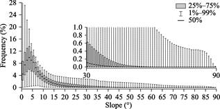
Figure 3 Box
chart of 22,205 DEM tiles slope frequency
distribution
|
4.3 Data Validation
|
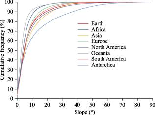
Figure
4
Cumulative frequency
distributions of slope in 7 continents and the total Earth land surface
|
The slope frequency distribution is a quantitative
analytical tool for slope analysis. However, slope accuracy depends on the DEM
data. The ASTER GDEM v3.0 data were created from the automated processing of
the entire ASTER Level 1A archive of scenes acquired
between March 1, 2000, and November 30, 2013. The ASTER GDEM Version 3 data products
offer a substantial improvement over Version 2 products[19].
Although some relief changes during the data acquisition period, on a global
scale the impact of these local topographic changes can be ignored. Figure 2 shows that Antarctica and Greenland have a high
ground surface slope. Because ice and snow-covered areas
have high optical reflectivity, a stereo correlation was used to produce the ASTER DEM. Therefore, DEM data in this area have poor quality and so
do the slope frequency distribution data. We suggest that the slope frequency
distribution data for Antarctica and Greenland in this data set be avoided in
subsequent research.
Table 2 Land slope frequency distribution for different
statistic units
|
Statistic unit
|
Mean value
?? (??)
|
Standard deviation
?? (??)
|
Statistic unit
|
Mean value
?? (??)
|
Standard deviation
?? (??)
|
|
Africa
|
6.25
|
5.38
|
South America
|
8.25
|
7.77
|
|
Asia
|
9.63
|
9.34
|
Oceania
|
5.23
|
5.31
|
|
Europe
|
7.70
|
6.98
|
Antarctica
|
13.53
|
15.86
|
|
North America
|
9.43
|
10.74
|
Earth
|
8.63
|
9.28
|
5 Discussion and Conclusion
|
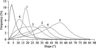
Figure 5 Slope frequency
distributions from previous studies (dash line) and a global land slope
distribution (solid line) 1??Lucore hollow a mature basin[1]; 2??the
Northwestern Himalayas[12]; 3??wash number is 4 mm??yr‒1
throughout the continental United States[8]; 4??wash number is
8mm??yr‒1 throughout the continental United States[8];
5??wash number is 16 mm??yr‒1 throughout the continental United
States[8]; 6??landslide areas in Upper Tiber River basin[21]
|
We
suggest that slope frequency distributions
vary between the study areas and the size and landforms of the study areas[1,8,12,21]. Slope distributions significantly
vary (dash line, Figure 5); hence, we can neither compare across
regions nor compare with statistical models. However, if compared with a global
land slope frequency distribution (solid line, Figure 5), we can easily and quantitatively describe ground
slope in a global uniform context. For example, the peak slope of curve 6 in Figure
5 is the closest to the global land peak
slope, indicating that the terrain slope of the study area is relatively
gentle. Similarly, the terrain slope of the study area represented by curve 5
is the most rugged.
The slope is a strong scale-dependent parameter that
cannot be compared across different DEM resolutions. To date, few studies of
global slope frequency distribution have been conducted at high resolution. As
a useful parameter in earth sciences, which can provide quantitative
characteristics for describing ground surfaces, the global slope frequency distribution
needs to match the common 30 m DEM resolution. 30 m is one of the common free
DEM resolutions. The slope frequency distribution generated from ASTER GDEM
v3.0 can provide a global reference for slope frequency analysis (e.g.
landslide, geomorphic). This dataset includes land slope frequency
distributions for 3 statistical units: 1?? (latitude) ´ 1?? (longitude) grids, the 7 continents, and the
entire globe, that enrich regional and global benchmarks. We hope this suite of
land slope frequency distributions will facilitate future quantitative
cross-region slope analysis at the 30 m resolution. Because slope frequency distribution
data might vary for different DEMs generated from different data sources, this data set can only be used as a reference
for studies based on GDEM v3.0 data.
Author Contributions
Peng, Q. Z. designed the dataset processing. Tang, L. and
Ma, J. W. designed the algorithms for the dataset. Ma, J. W. and Shao, Z. Y.
contributed to data processing and analysis. Tang, L. wrote the data paper.
References
[1]
Strahler, A.
N. Quantitative slope analysis [J]. Geological
Society of America Bulletin, 1956, 67(5): 571-596.
[2]
Sharpton, V.
L., Head, J. W. Analysis of regional slope characteristics on Venus and Earth [J].
Journal of Geophysical Research: Solid Earth, 1985, 90(B5): 3733?C3740.
[3] Aharonson, O., Zuber, M. T., Neumann, G. A., et al. Mars: northern hemisphere slopes
and slope distributions [J]. Geophysical
Research Letters, 1998, 25(24): 4413-4416.
[4]
Thomson, B.
J., Head III, J. W. Utopia Basin, Mars: characterization of topography and
morphology and assessment of the origin and evolution of basin internal
structure [J]. Journal of Geophysical
Research: Planets, 2001,
106(E10): 23209-23230.
[5]
Yan, Y. Z.
Research on lunar slope spectrum variations based on digital elevation models [D].
Nanjing: Nanjing Normal University, 2015.
[6]
Montgomery,
D. R. Slope distributions, threshold hillslopes, and steady-state topography [J].
American Journal of Science, 2001,
301(4/5): 432-454.
[7] DiBiase, R. A, Heimsath, A. M., Whipple, K. X.
Hillslope response to tectonic forcing in threshold landscapes [J]. Earth Surface Processes and Landforms,
2012, 37(8): 855-865.
[8] Wolinsky, M. A., Pratson, L. F. Constraints on
landscape evolution from slope histograms [J]. Geology, 2005, 33(6): 477-480.
[9]
Peng, Q. Z.,
Tang, L., Chen, J., et al. Study on
the evolution of construction land slope spectrum in Shenzhen during 2000‒2015 [J].
Journal of Natural Resources, 2018,
33(12): 2200-2212.
[10] O??Neill, M. P., Mark, D. M. On the
frequency distribution of land slope [J]. Earth
Surface Processes and Landforms, 1987, 12(2): 127-136.
[11] Tang, G., Song, X., Li, F., et al. Slope spectrum critical area and its spatial variation in
the Loess Plateau of China [J]. Journal
of Geographical Sciences, 2015, 25(12): 1452-1466.
[12] Burbank, D. W, Leland, J., Fielding, E., et al. Bedrock incision, rock uplift,
and threshold hillslopes in the northwestern Himalayas [J]. Nature, 1996, 379(6565): 505.
[13] Iwahashi, J., Watanabe, S., Furuya, T. Mean
slope-angle frequency distribution and size frequency distribution of landslide
masses in Higashikubiki area, Japan [J]. Geomorphology,
2003, 50(4): 349-364.
[14] Zhao, S., Cheng, W. Transitional relation
exploration for typical loess geomorphologic types based on slope spectrum
characteristics [J]. Earth Surface
Dynamics, 2014, 2(2): 433-441.
[15]
Zhou, Q.,
Liu, X. Analysis of errors of derived slope and aspect related to DEM data
properties [J]. Computers &
Geosciences, 2004, 30(4): 369-378.
[16]
Tachikawa,
T., Hato, M., Kaku, M., et al.
Characteristics of ASTER GDEM version 2 [C]. 2011 IEEE international geoscience
and remote sensing symposium. IEEE, 2011: 3657-3660.
[17]
Tang, L.,
Ma, J. W., Shao, Z. Y., et al. Global
land slope frequency dataset [DB/OL]. Global Change Data Repository, 2020. DOI:
10.3974/geodb.2020.02.02.V1.
[18]
GCdataPR
Editorial Office. GCdataPR data sharing policy [OL]. DOI:
10.3974/dp.policy.2014.05 (Updated 2017).
[19]
NASA, METI.
ASTER GDEM v3.0 [Z]. https://lpdaac.usgs.gov/.
[20]
Tachikawa,
T., Manabu, K., Akira, I. ASTER GDEM Version 3 validation report [Z]. NASA,
2015.
[21]
Guzzetti, F.,
Ardizzone, F., Cardinali, M., et al.
Distribution of landslides in the Upper Tiber River basin, central Italy [J]. Geomorphology, 2008, 96(1): 105-122.