A Satellite-Based Dataset of Global Atmospheric Carbon
Dioxide Concentration with a Spatial Resolution of 2?? ?? 2.5?? from 1992 to 2020
Hou, W. Y.1 Jin, J. X. 1,2* Yan, T. 1 Liu, Y.1
1. College of Hydrology and
Water Resources, Hohai University, Jiangsu, Nanjing 210024, China;
2. National Earth System Science Data Center, National Science
& Technology Infrastructure of China, Beijing 100101, China
Abstract: Carbon dioxide (CO2) is one of the
main greenhouse gases in the atmosphere. It plays a crucial role in global
climate change, of which temporal and spatial patterns have been paid great
attention to. Taking CO2 concentration as the research object, this
study developed a global gridded dataset of monthly CO2
concentration with a spatial resolution of 2?? ?? 2.5?? from 1992 to 2020. The time series of CO2
concentration was simulated by an improved sinusoidal model, which was
calibrated by the remotely-sensed product of tropospheric CO2
concentration from 2002 to 2012 (AIR??3C2M
005), for each grid cell. Then, field-observed data of CO2
concentration were adopted to evaluate the accuracy of our product. The results
showed that: (1) the CO2 concentration of our production was highly
consistent with that observed at the stations. Especially, it performed well in
the fitting (2002–2012: R2
= 0.94, RMSE = 1.34 ppm), reconstruction (1992–2001: R2
= 0.92, RMSE = 1.50 ppm) and prediction (2013–2019: R2
= 0.93, RMSE = 1.58 ppm) of CO2 concentration, respectively. (2) our data showed that
the global atmospheric CO2 concentration exhibited an obvious
spatial heterogeneity. The high value regions of CO2 concentration
were mainly located in the northern of North America, while the low values
dominated middle latitudes of the southern hemisphere.
Keywords: carbon
dioxide; remote sensing; simulation; AIRS; global
DOI: https://doi.org/10.3974/geodp.20146.14.2022.02.04
CSTR: https://cstr.escience.org.cn/CSTR:20146.14.2022.02.04
Dataset Availability Statement:
The dataset
supporting this paper was published and is accessible through the Digital Journal of Global Change Data
Repository at: https://doi.org/10.3974/geodb.2021.11.01.V1 or
https://cstr.escience.org.cn/CSTR:20146.11.2021.11.01.V1.
1 Introduction
With
the global economy development, a great deal of fossil fuels has been used
which leads to a significant increase in carbon dioxide (CO2)
emissions. It has a great impact on the global climate, ecosystems and economic
fields. The Intergovernmental Panel on Climate Change (IPCC) Fifth Assessment
Report (AR5) states that CO2 and methane are the main contributors
to global warming (about 88%–90%)[1]. As an important greenhouse
gas, the increase in the atmospheric concentration of CO2 has a
significant heating effect on the ground[2,3], which has attracted
widespread attention from government departments and the scientific community.
Exploring, retracing and predicting the changes of CO2 concentration
over the world are of great practical significance to adopt targeted policies
and measures dealing with global climate change issues and achieving
sustainable socio-economic developments.
Currently, there
are three main ways to obtain CO2 observations: ground-based,
space-based and satellite remote sensing observations[4]. Data from
ground-based stations have a large time span and high accuracy, which can be
used as a benchmark for satellite observations. Many scholars used single-site
data to represent the global CO2 concentrations, which performed
well in the studies. However, given the spatial heterogeneity of CO2
distribution, single-site data was insufficient to present the truth on a
global scale. In addition, ground observation stations are set up in sparsely
populated and complex terrain. There are defects, e.g., the difficult
construction, high cost of maintenance, small coverage, uneven distribution.
Moreover, many sites are needed to cooperatively explore the regional dynamic
change of CO2[5,6]. Although CO2 concentration
can be measured with high accuracy, it had certain limitations for obtaining
global CO2 concentration data. Space-based exploration used aircraft
or hot air balloons to make real-time high-altitude CO2
concentration measurements in areas designated by the Earth System Research
Laboratory (ESRL)[7,8]. Compared with site observations, CO2
measurement data with a wider spatial coverage could be obtained through this
method. However, due to the high cost of equipment and low timeliness,
space-based detection could not acquire data continuously for a long time.
Remote sensing uses diverse sensors on board satellites to acquire the spectral
characteristics of atmospheric CO2 which are radiated by the sun and
reflected back into space through the ground. Tropospheric CO2
observations with long-term, continuous, spatiotemporal consistency and high
accuracy could be provided for continents and oceans[9]. This view
has been widely accepted by the academic community. Currently, the atmospheric
data provided by the Atmospheric Infrared Sounder (AIRS) have been adopted by
many scholars in studies of atmospheric CO2. With 2378 continuous
infrared spectral channels (3.7–15.4 ??m), the AIRS receives accurate infrared
spectral data of land, ocean and atmosphere, and provides many hyperspectral
and high-precision data including parameters of temperature, humidity, clouds,
surfaces, and CO2[10]. By comparing the AIRS data with
the sounding observations, Divakarla et al. found that the relative error
between land and sea did not exceed 10%[11]. Since the process of
transporting surface CO2 to the atmospheric troposphere one takes a
few time, the data of AIRS inversion lags behind the real CO2
concentration. Satellite CO2 data products were derived from the
near-infrared spectrum, in which they were strongly disturbed by surface
atmospheric aerosols. This results in that global CO2 data inversion
by AIRS have a high degree of confidence only in the middle and lower layers of
the troposphere[12]. It is urgent to develop a set of global-scale,
longtime series, and high-precision CO2 concentration data to
support global change studies.
In these views, a
new satellite-based dataset of global atmospheric CO2 concentration
was developed using an improved sinusoidal model in this study, including
monthly and annual mean CO2 concentration over the world. First, in
order to ensure that satellite remote sensing data can accurately capture the
concentration of tropospheric CO2, the AIRS satellite remote sensing
inversion data was validated by ground station observed data. Second, based on
the improved sinusoidal model, the model was parameterized for each grid cell,
and the global CO2 simulation was carried out. The simulation
results were evaluated by both site observations and satellite data, so that to
provide reliable data of global CO2 change.
2 Metadata of the Dataset
The
metadata of the dataset [13] is summarized in Table 1. It includes
the dataset full name, short name, authors, year of the dataset, temporal
resolution, spatial resolution, data format, data size, data files, data
publisher, and data sharing policy, etc.
Table 1 Metadata summary of the Global
atmospheric carbon dioxide concentration simulation grid dataset (1992‒2020)
|
Items
|
Description
|
|
Dataset full name
|
Global
atmospheric carbon dioxide concentration simulation grid dataset (1992‒2020)
|
|
Dataset short
name
|
GlobalSimulatedCO2_1992‒2020
|
|
Authors
|
Hou, W. Y.
ABE-5925-2021, Hohai University, houhh5425@163.com
Jin, J. X.
ABE-5853-2021, Hohai University, jiaxinking@hhu.edu.cn
|
|
|
Yan, T.
ABE-5824-2021, Hohai University, 191309010014@hhu.edu.cn
Liu, Y.
ABE-5924-2021, Hohai University, 201301060011@hhu.edu.cn
|
|
Geographical
region
|
60??S–88??N??180??W–180??E
|
Year
|
1992–2020
|
|
Temporal
resolution
|
Monthly CO2
concentration from 1992 to 2020; annual mean CO2 from 1992 to 2020
|
|
Spatial
resolution
|
2?? ?? 2.5?? (Lat ?? Long)
|
Data format
|
NetCDF (.nc)
|
|
Data size
|
23.9 MB (After compression)
|
|
|
Data files
|
(1) Global monthly
mean dataset of CO2 concentrations during 1992–2020
(2) Global annual
mean dataset of CO2 concentrations during 1992–2020
|
|
Foundations
|
Ministry
of Science and Technology of P. R. China (2018YFA0605402); National
Natural Science Foundation (41971374)
|
|
Data publisher
|
Global Change Research Data Publishing & Repository,
http://www.geodoi.ac.cn
|
|
Address
|
No. 11A, Datun
Road, Chaoyang District, Beijing 100101, China
|
|
Data sharing
policy
|
Data from the Global
Change Research Data Publishing & Repository includes metadata, datasets (in the Digital Journal of Global Change Data Repository), and
publications (in the Journal of Global Change Data & Discovery). Data sharing policy includes: (1) Data are openly
available and can be free downloaded via the Internet; (2) End users are
encouraged to use Data subject to citation; (3) Users, who are by definition
also value-added service providers, are welcome to redistribute Data
subject to written permission from the GCdataPR Editorial Office and the
issuance of a Data redistribution license; and (4) If Data are used to
compile new datasets, the ??ten per cent principal?? should be followed such
that Data records utilized should not surpass 10% of the new
dataset contents, while sources should be clearly noted in suitable places in
the new dataset[14]
|
|
Communication and searchable system
|
DOI, CSTR, Crossref, DCI, CSCD,
CNKI, SciEngine, WDS/ISC, GEOSS
|
|
|
|
|
|
3 Data Development Methodology
3.1 Data Sources
In
this paper, the tropospheric CO2 data product (AIRS ?? 3C2M005)
jointly retrieved by AIRS and the Advanced Microwave Sounding Unit (AMSU) was
used as the reference data to produce the global CO2 concentration
dataset. AIRS/AMSU/HSB (the Humidity Sounder for Brazil) is a set of advanced
atmospheric vertical profile observation instruments from infrared to microwave
band, which is used to measure atmospheric temperature and provide information
of atmospheric water vapor distribution, data of cloud, sea, land temperature
and atmospheric humidity[15]. The adopted data was the third-level
monthly average CO2 data (version 5). The spatial coverage of the
data is 60??S–90??N with a spatial resolution of 2?? ?? 2.5?? (latitude ??
longitude). The data was downloaded from the Goddard Earth Sciences Data and
Information Services Center (GES DISC) of the National Aeronautics and Space
Administration (NASA). In addition, the tropospheric CO2 data
product during 2010–2017 (AIRS3C2M 005) retrieved from AIRS was used to compare
with the simulated data and site observations.
In our study, the
AIRS remote sensing data and the products were evaluated by the monthly average
CO2 data of the stations. Seven sites were selected, namely Samoa
(SMO), Mouna Loa (MLO), Variguan (WLG), Asserkrem (ASK), Niwot Ridge (NWR),
Monte Cimone (CMN), and Plateau Rose (PRS) (Figure 1). The site data were
obtained from the World Data Center for Greenhouse Gases (WDCGG). The global
monthly average CO2 data was downloaded from the Global Monitoring
Laboratory of the National Oceanic and Atmospheric Administration (NOAA GML).
3.2 Algorithm Principle
The
improved sinusoidal model[15] proposed by the Carbon Cycle Team of
NOAA GML was adopted in this study. The model can reduce the noise generated
from the process of estimating the global value due to atmospheric variability
at the weather scale and measurement time gap.
The weekly air
sample data from the global air sampling network[16] were used by
Carbon Cycle Team of NOAA GML to calculate the global
average surface value[17–20]. The samples came from the marine
boundary layer (MBL) with well atmospheric mixing. The data could be estimated
directly without the atmospheric transmission model, which captures the
global trend with low noise. Global CO2 concentration showed an upward
trend and fluctuated with season. So, NOAA GML stakeholders chose a combination
of quadratic functions and sine and cosine functions to represent suitably
smooth curves for the MBL data. The specific parameters of the model vary with
the gas type, site, and sampling frequency[15].The calculation
formula is as follows:
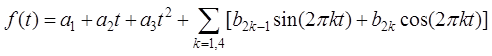 (1)
(1)
where t
denotes time. The model contains three polynomial parameters a1,
a2, a3, and eight sine and cosine harmonic
parameters b2k-1 and b2k (k = 1,2,3,4).
The model was applied to AIRS and AMSU satellite data
products, and the consistency between the simulated data and satellite data was
evaluated to ensure whether the model was also suitable. The AIRS and AMSU
satellite data was input into the model, and the parameters were determined for
each cell in the range of 60??S–88??N. Then, the simulation was performed to
obtain the CO2 concentration dataset pixel by pixel for this range.
In order to analyze the interannual trend of CO2 concentration from
1992 to 2020, the annual average growth trend of global CO2
concentration was estimated by using Sen??s slope estimator. That is, the median
slope of all lines of paired points was selected as the slope overall. This
method could effectively calculate the change trend and reduce the uncertainty
caused by outliers.
4 Data Results and Validation
4.1 Data description
The
dataset mainly contents two subsets: (1) Global monthly mean CO2
concentration dataset during 1992–2020, which includes 29 data files, named as
CO2_mon_****.nc. (2) Global annual mean CO2 concentration
dataset during 1992–2020, which includes 29 data files, named as CO2_mean_****.nc.
4.2 Spatial and Temporal Variabilities of the CO2
Concentration
The
spatial distribution of the average CO2 concentration data over the
world from 1992 to 2020 is shown in Figure 1. Generally, the distribution of CO2
exhibited an obvious spatial heterogeneity. The CO2 concentration in
the northern hemisphere was generally higher than that in the southern
hemisphere. The areas with high CO2 concentration were mainly
distributed in northern North America, eastern Asia and low latitudes of the
northern and southern hemispheres, while the areas with low CO2
concentration were mainly distributed in the middle and high latitudes of the
southern hemisphere and parts of Siberia.
Figure 2 shows the global pattern of the
interannual trend of annual average CO2 concentration from 1992 to
2020. Global CO2 concentration is increasing, but the growth rate
shows spatial heterogeneity. Overall, the growth rate of CO2
concentration in the northern hemisphere was faster than that in the southern
hemisphere. The CO2 concentration in the high latitudes of the
northern hemisphere, such as Siberia and northern North America, was increasing
rapidly. In contrast, the areas with a slower rate were mainly located in the
northern South America, central Africa and the low latitudes of the southern
and northern hemispheres.
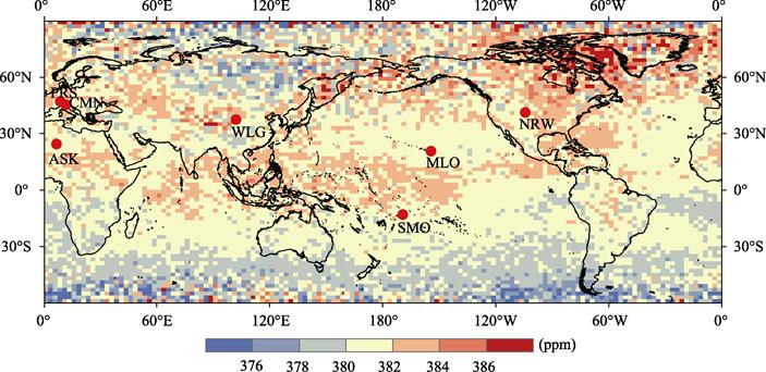
Figure
1 Spatial distribution of the multi-year mean CO2
concentration from 1992 to 2020
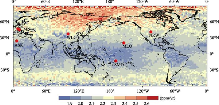
Figure
2 Spatial distribution of the trends in
annual average CO2 concentration from 1992 to 2020
4.3 Data Validation
4.3.1 Comparison of Fitting Results with
Site Data
The simulation of
CO2 concentration in this study was compared with that from the
seven stations from 1992 to 2019 (Figure 3). The result showed a significant
linear relationship between them, indicating that the fitting results were well
consistent with the concentration of CO2 on the ground.
|

Figure
3 Comparison between the observed and
simulated CO2 concentration data at the seven stations
(Notes: SMO,
Samoa; MLO, Mouna Loa; WLG, Variguan; ASK, Asserkrem; NWR, Niwot Ridge; CMN, Monte
Cimone; PRS, Plateau Rose, and the same below.)
|
Performances of the proposed CO2 concentration in
this study were investigated in the reconstruction (1992‒2001), fitting
(2002‒2012) and prediction (2013‒2019) phases, respectively, including
correlation coefficient, root mean square error (RMSE) and average relative
error between the observed and simulated data at the seven stations (Table
2–4). The results showed that this dataset was well consistent with the observed CO2 concentration on the ground
in each phase. The error between the observed and simulated data in the fitting
phase was the smallest, and RMSE was less than 5 ppm, which can well represent
the ground CO2 concentration.
4.3.2 Comparison of Fitting Results,
Satellite Data and Station Data
Three datasets of
CO2 concentration, i.e., the simulated data of this study, the AIRS
product (2010.01–2017.02) and the site observations, were further compared
using correlation coefficient (r), RMSE, relative error and R2 at the seven stations. The
results showed that the consistency between our simulated data and the observed
data was generally better than that between the AIRS data and the observed
data, indicating our dataset can well represent the real CO2
concentration.
Table 2 Comparison between the observed and
simulated monthly average CO2 concentration in the reconstruction
phase (1992–2001)
|
Site
|
Mean value (ppm)
|
Average
deviation
(ppm)
|
Correlation
coefficient
|
RMSE
(ppm)
|
Relative error
|
|
Observed
|
Simulated
|
|
SMO
|
362.88
|
362.78
|
0.10
|
0.994,4
|
0.91
|
0.20%
|
|
MLO
|
364.33
|
361.73
|
2.60
|
0.969,0
|
2.98
|
0.72%
|
|
WLG
|
365.86
|
362.96
|
2.90
|
0.845,8
|
2.71
|
0.63%
|
|
ASK
|
367.39
|
359.97
|
7.43
|
0.922,5
|
3.67
|
0.87%
|
|
NWR
|
364.78
|
360.58
|
4.20
|
0.913,4
|
5.22
|
1.22%
|
|
CMN
|
364.22
|
362.98
|
1.24
|
0.772,7
|
4.83
|
1.21%
|
|
PRS
|
364.65
|
363.64
|
1.02
|
0.877,7
|
2.94
|
0.69%
|
Table 3 Comparison between the observed and
simulated monthly average CO2 concentration in the simulation phase
(2002–2012)
|
Site
|
Mean
value (ppm)
|
Average
deviation
(ppm)
|
Correlation
coefficient
|
RMSE
(ppm)
|
Relative error
|
|
Observed
|
Simulated
|
|
SMO
|
381.79
|
382.70
|
‒0.91
|
0.997,3
|
0.90
|
0.21%
|
|
MLO
|
383.66
|
382.00
|
1.66
|
0.970,6
|
2.21
|
0.49%
|
|
WLG
|
383.63
|
382.57
|
1.05
|
0.944,3
|
2.58
|
0.57%
|
|
ASK
|
383.42
|
382.78
|
0.64
|
0.954,7
|
1.99
|
0.46%
|
|
NWR
|
384.22
|
383.58
|
0.64
|
0.916,2
|
2.64
|
0.61%
|
|
CMN
|
383.23
|
384.22
|
‒0.99
|
0.780,6
|
4.65
|
1.06%
|
|
PRS
|
383.69
|
383.78
|
‒0.10
|
0.884,9
|
3.04
|
0.67%
|
Table 4 Comparison between the
observed and simulated monthly average CO2 concentration in the
prediction phase (2013–2019)
|
Site
|
Mean
Value (ppm)
|
Average
deviation (ppm)
|
Correlation
coefficient
|
RMSE
(ppm)
|
Relative error
|
|
Observed
|
Simulated
|
|
SMO
|
400.63
|
399.92
|
0.70
|
0.996,1
|
1.39
|
0.28%
|
|
MLO
|
402.97
|
401.88
|
1.09
|
0.968,8
|
1.86
|
0.40%
|
|
WLG
|
402.99
|
400.44
|
2.55
|
0.925,0
|
3.68
|
0.78%
|
|
ASK
|
402.78
|
400.85
|
1.93
|
0.951,1
|
3.00
|
0.61%
|
|
NWR
|
403.43
|
401.91
|
1.52
|
0.898,8
|
3.31
|
0.71%
|
|
CMN
|
403.37
|
402.75
|
0.62
|
0.718,9
|
5.02
|
1.09%
|
|
PRS
|
401.35
|
403.87
|
–2.52
|
0.832,3
|
3.65
|
0.68%
|
5 Discussion and Summary
|
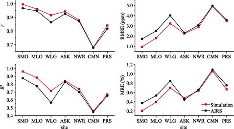
Figure 4 Comparison among the CO2
concentration data derived from the simulated product of this study,
satellite data products (AIRS) and site observations
|
It
was found that there may be a large deviation between the simulated and
observed results. So, it is necessary to determine a starting point in order to
ensure the good consistency between the backtracking results and the site
observations. The growth trend of CO2 in each region were generally
consistent with that of the global average CO2. Hence, the global
average CO2 (1980–2019) was used as the reference data. Since
1985, it had been calculated and compared as a segmentation point year by year. The time before and after the segmentation point was parameterized
and simulated respectively, and then its results were compared consistently
with the global average to ensure the highest accuracy.
After inspection, when 1992 was taken as the segmentation point, the R2
of the simulation was the highest (0.999,5) and RMSE was the lowest (0.451
ppm). Therefore, the year of 1992 was adopted as the starting year of this
dataset.
|
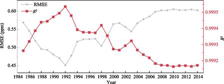
Figure 5 Comparison of
consistency between simulation results and global observation data before and
after different years as turning points
|
The global
tropospheric CO2 concentration product jointly derived from AIRS and
AMSU was used as reference data for parameter calibration of the improved
sinusoidal estimation model and simulation of CO2 concentration
pixel by pixel. Then, field-observed
data of CO2 concentration were adopted to validate and evaluate the
accuracy of our product. The dataset shows that the atmospheric CO2 concentration
exhibited an obvious spatial heterogeneity over the world. The high value
regions of CO2 concentration were mainly located in the middle and
high latitudes of the northern hemisphere, and the low values dominated low
latitudes of the southern hemisphere. Comparing the dataset with the site
observation data, it is found that the two sets of data performed well in backtracking,
simulation and prediction phases, which can well represent the spatio-temporal
distribution global CO2 in a long time series. Compared with the
original satellite remote sensing data, this dataset can be used to study the
change of atmospheric CO2 concentration in a longer time series.
Furthermore, it can improve the limitation that single-site numerical value was
used to represent global CO2 concentration in modeling at a global
scale, and provide data support for studies of geography, ecology and other
disciplines.
Author Contributions
Jin, J.
X. made an overall design of this study; Hou, W. Y. collected and processed the
data, and wrote the paper. Yan, T. wrote the codes. Liu, Y. verified the data
of the paper.
Conflicts of
Interest
The
authors declare no conflicts of interest.
References
[1]
Hartmann, D. L., Klein Tank, A. M. G., Rusticucci,
M., et al. IPCC Climate Change 2013: The Physical Science Basis, Contribution
of Working Group I to the Fifth Assessment Report of the Intergovernmental Panel
on Climate Change [M]. Cambridge: Cambridge University Press, 2013.
[2]
Callendar, G. S. The artificial
production of carbon dioxide and its influence on temperature [J]. Quarterly
Journal of the Royal Meteorological Society, 1938, 64(275): 223–240. DOI: 10.1002/qj.49706427503.
[3]
Bacastow, R. B. The effect of
temperature change of the warm surface waters of the oceans on atmospheric CO2
[J]. Global Biogeochemical Cycles, 1996, 10(2): 319‒333.
[4]
Qianwen, M., Qiu Y. Remote
sensing analysis of multi-years spatial and temporal variation of CO2
in China [J]. Remote Sensing Technology and Application, 2016, 31(2):
203‒213.
[5]
Bergamaschi, P., Frankenberg,
C., Meirink, J. F., et al. Inverse modeling of global and regional CH4
emissions using SCIAMACHY satellite retrievals [J]. Journal of Geophysical
Research: Atmospheres,
2009, 114: D22301. DOI: 10.1029/2009JD012287.
[6]
Shi, G. Y., Dai, T., Xu, N.
Latest progress of the study of atmosphere CO2 concentration
retrievals from Satellite [J]. Advances in Earth Science, 2010 (1):
7‒13.
[7]
Menzel, W. P., Schmit, T. J.,
Zhang, P., et al. Satellite-based atmospheric infrared sounder
development and applications [J]. Bulletin of the American Meteorological
Society, 2018, 99(3):
583–603. DOI: 10.1175/ BAMS-D-16-0293.1.
[8]
Machida, T., Matsueda, H.,
Sawa, Y., et al. Worldwide measurements of atmospheric CO2
and other trace gas species using commercial airlines [J]. Journal of
Atmospheric and Oceanic Technology, 2008, 25(10): 1744–1754. DOI: 10.1175/2008JTECHA1082.1.
[9]
Liu, Y., Lv, D. R., Chen, H.
B., et al. Advances in technologies and methods for satellite remote
sensing of atmospheric CO2 [J]. Remote Sensing Technology and
Application, 2011, 26(2): 247‒254.
[10]
Kuze, A., Suto, H., Nakajima, M., et al. Thermal and near
infrared sensor for carbon observation Fourier-transform spectrometer on the
Greenhouse Gases Observing Satellite for greenhouse gases monitoring [J]. Applied
optics, 2009, 48(35): 6716–6733. DOI: 10.1364/AO.48.006716.
[11]
Divakarla, M. G., Barnet, C. D., Goldberg, M. D., et al. Validation of
Atmospheric Infrared Sounder temperature and water vapor retrievals with
matched radiosonde measurements and forecasts [J]. Journal of Geophysical
Research: Atmospheres,
2006, 111: D09S15. DOI: 10.1029/2005JD006116.
[12]
Zhou, M. D. Atmospheric carbon dioxide (CO2) retrieval and
sensitivity studies from satellite observations [D]. Shanghai: East China Normal University, 2013.
[13]
Hou, W. Y., Jin, J. X., Yan,
T., et al. Global
atmospheric carbon dioxide concentration simulation grid dataset (1992–2020) [J/DB/OL]. Digital Journal of
Global Change Data Repository,
2021. https://doi.org/10.3974/geodb.2021.11.01.V1. https://cstr.escience.org.cn/CSTR:20146.11.2021.11.01.V1.
[14]
GCdataPR Editorial Office.
GCdataPR data sharing policy [OL]. https://doi.org/10.3974/dp.policy.2014.05
(Updated 2017).
[15]
Thoning, K. W., P. P. Tans and
W.D. Komhyr, Atmospheric Carbon Dioxide at Mauna Loa Observatory 2. Analysis of
the NOAA GMCC Data, 1974–1985 [J]. Journal
of Geophysical Research: Atmospheres,
1989, 94(D6): 8549–8565.
[16]
Fetzer, E., Mcmillin, L. M.,
Tobin, D., et al. AIRS/AMSU/HSB validation [J]. IEEE transactions on
geoscience and remote sensing, 2003, 41(2): 418–431.
DOI:10.1109/TGRS.2002.808293.
[17]
Conway, T. J., Tans, P. P.,
Waterman, L. S., et al. Evidence for interannual variability of the
carbon cycle from the National Oceanic and Atmospheric Administration/Climate
Monitoring and Diagnostics Laboratory global air sampling network [J]. Journal
of Geophysical Research:
Atmospheres, 1994, 99(D11): 22831–22855. DOI: 10.1029/94JD01951.
[18]
Dlugokencky, E. J., Steele, L.
P., Lang, P. M., et al. The growth rate and distribution of atmospheric
methane [J]. Journal of Geophysical Research: Atmospheres, 1994, 99(D8): 17021–17043. DOI: 10.1029/ 94JD01245.
[19]
Novelli, P. C., Steele, L. P.,
Tans, P. P. Mixing ratios of carbon monoxide in the troposphere [J]. Journal
of Geophysical Research: Atmospheres, 1992, 97(D18): 20731–20750. DOI: 10.1029/92JD02010.
[20]
Trolier, M., White, J. W. C.,
Tans, P. P., et al. Monitoring the isotopic composition of atmospheric
CO2: Measurements from the NOAA Global Air Sampling Network [J]. Journal of
Geophysical Research: Atmospheres, 1996, 101(D20): 25897–25916. DOI: 10.1029/96JD02363.