Equity Dataset Development of PM_2.5 Exposure for Different Population Groups in Six Cities of China from the Trajectory Data Perspective

WU Zihao^1,2  MA Zhifeng^1,2  XIA Jizhe^1,2*

1. School of Architecture and Urban Planning, Shenzhen University, Ministry of Natural Resources (MNR) Key Laboratory for Geo-Environmental Monitoring of Great Bay Area, Guangdong Key Laboratory of Urban Informatics, Shenzhen Key Laboratory of Spatial Smart Sensing and Service, Shenzhen 518060, China;

2. State Key Laboratory of Subtropical Building and Urban Science, Shenzhen 518060, China

Abstract: The authors calculated individual hourly average PM_2.5 exposure concentrations by overlaying cleaned large-scale population trajectory data with hourly 1-km resolution PM_2.5 distribution data. Distinct from traditional static population distribution assumptions, this method more accurately reflects individual PM_2.5 exposure levels across different spatiotemporal contexts. The study computed the hourly average PM_2.5 exposure concentrations for groups differentiated by gender, age, income, and commuting distance. Based on this, the Gini coefficient of resident exposure and the concentration index for different groups in each city were evaluated, systematically identifying vulnerable groups and spatial inequality patterns of PM_2.5 exposure across cities. We established a dataset of PM_2.5 exposure equity for different population groups based on trajectory data. This dataset includes the following data for the study area from January 24 to February 23, 2023: (1) Hourly 1-km spatial distribution data of PM_2.5 concentration for 6 cities including Beijing, Shanghai, and Shenzhen; (2) Urban per capita PM_2.5 exposure concentration based on dynamic mobile phone trajectories; (3) Hourly average PM_2.5 exposure data for groups with different social characteristics (age, income, and gender) and spatial characteristics (commuting distance) in each city; (4) Gini coefficient of PM_2.5 exposure for residents in each city; (5) Results of OLS regression analysis of the PM_2.5 exposure concentration index for various groups; (6) County-level hourly average PM_2.5 exposure amount for residents. The dataset is archived in .shp, .tif, and .xlsx formats, comprising 753 data files with a total data volume of 10.6 GB (compressed into one file, 127 MB).

Keywords: GPS trajectory data; PM_2.5 concentration retrieve; PM_2.5 exposure assessment; inequality analysis

DOI: https://doi.org/10.3974/geodp.2026.02.08

Dataset Availability Statement:

The dataset supporting this paper was published and is accessible through the Digital Journal of Global Change Data Repository at: https://doi.org/10.3974/geodb.2026.02.08.V1

1 Introduction

Entering the 21st century, accompanied by rapid urbanization and industrialization, the issue of PM_2.5 pollution in China has become increasingly prominent. Air pollution, especially PM_2.5, has been strongly linked to various health problems^[1,2]. Existing research^[3] indicates that long-term exposure to high concentrations of PM_2.5 can lead to premature mortality. Therefore, proactive air pollution prevention and control are essential. To address the issue of PM_2.5 pollution, China explicitly included PM_2.5 concentration in the expanded pollutant standards in the Ambient air quality standards (GB3095—2012) published in 2012^[4].

Current analyses of PM_2.5 exposure equity differences mostly rely on census statistical data^[5–7], with the core assumption that individuals are located within static residential spaces, using the regional average PM_2.5 concentration as the exposure level for all residents in that area. This method ignores the impact of individual daily mobility on air pollution exposure, making it difficult to reflect dynamic and realistic exposure risk distributions, thereby introducing bias in environmental equity assessments. PM_2.5 exposure equity refers to whether the distribution of PM_2.5 pollution exposure levels is fair among different social groups, such as those characterized by varying income, age, gender, and commuting distance. If the average exposure concentration of one group is significantly higher than that of others, it indicates the existence of exposure inequality.

By combining high spatiotemporal resolution PM_2.5 data with group trajectory data, this dataset enables a more comprehensive understanding of the differences in PM_2.5 exposure among different social groups and the underlying reasons. Such integrated analysis not only elucidates the impact of air pollution on public health but also provides a scientific basis for formulating targeted air quality management measures and public health policies.

2 Metadata of the Dataset

The metadata of 1-km hourly raster dataset of PM_2.5 exposure equality in six cities of China from the trajectory data perspective (Jan. –Feb. 2023)^[8] dataset is summarized in Table 1. It includes the dataset full name, short name, authors, year of the dataset, data format, data size, data files, data publisher, and data sharing policy, etc.

3 Methods

3.1 Data Sources

The remote sensing data used for PM_2.5 distribution simulation are as follows. Ground-level PM_2.5 monitoring data were obtained from the hourly real-time air quality monitoring data released by the China National Environmental Monitoring Centre[1]. Aerosol Optical Depth (AOD) data utilized the MCD19A2 product[2] from MODIS Terra and Aqua satellites, with a spatial resolution of 1 km, sourced from the NASA LAADS DAAC platform. Meteorological data, including hourly variables of wind speed, temperature, humidity, precipitation, boundary layer height, were extracted from the ERA5 reanalysis dataset[3] released by the European Centre for Medium-Range Weather Forecasts (ECMWF). Topographic data used the SRTM GL1 Digital Elevation Model (DEM)² with a spatial resolution of 30 m, sourced from NASA. Normalized Difference Vegetation Index (NDVI) employed the MODIS MOD13Q1 product with a spatial resolution of 250 m, sourced from NASA². Urban built-up area data (building footprints and road networks) were obtained through the Baidu Maps Open Platform[4] to characterize urban structure and human activity intensity. Based on these multi-source data, a Stacking ensemble learning model was constructed to achieve hourly 1-km PM_2.5 concentration spatiotemporal prediction, thereby supporting subsequent population exposure and equity assessments.

Table 1  Metadata summary of the 1-km hourly raster dataset of PM_2.5 exposure equality in six cities of China from the trajectory data perspective (Jan. –Feb. 2023)

The large-scale individual trajectory data used in this study were provided by Moxing Technology. These data capture and record user behavioral dynamics at regular high frequencies using various positioning technologies, such as Wi-Fi, Bluetooth, and GPS. The data cover the entire spatial extent of 6 cities: Beijing, Shanghai, Shenzhen, Chengdu, Wuhan, and Xi’an. The dataset includes anonymized user IDs, timestamps, positioning methods, and precise latitude and longitude information. To minimize the impact of fluctuations in residents’ daily mobility patterns on experimental error, this study selected trajectory data spanning one month, from January 24 to February 23, 2023. To fully reflect an individual’s daily PM_2.5 exposure scenario, individual trajectory data with at least 20 hours of valid positioning records were selected. The spatial accuracy of this trajectory data is within 1 m, and the temporal accuracy is within 1 h.

3.2 Algorithms

3.2.1 High Spatiotemporal Resolution PM_2.5 Distribution Simulation

To accurately assess the differences in PM_2.5 exposure among various population groups, high spatiotemporal resolution PM_2.5 concentration distribution data are required. This study proposes an hourly PM_2.5 prediction model based on Stacking ensemble learning, integrating multi-source remote sensing and urban big data to achieve estimation of PM_2.5 concentration at 1-km resolution with hourly updates.

This study constructed a two-layer Stacking ensemble model to capture the complex nonlinear relationships between PM_2.5 and various influencing factors, as shown in Figure 1. The first layer base learners selected were XGBoost^[10], Gradient Boosting Machine (GBM)^[11], and Random Forest (RF)^[12], all of which perform excellently in air quality prediction and can effectively handle high-dimensional heterogeneous data. The second layer meta-learner employed Elastic Net^[13], combining L1 and L2 regularization to avoid overfitting and enhance model generalization capability. Model training utilized five-fold cross-validation, and hyperparameters (such as learning rate, tree depth, regularization coefficients) were optimized independently for each city to adapt to regional characteristics.

This study selected relevant features based on correlation analysis, including AOD, NDVI, road network density, and other target features as independent variables for model training, with PM_2.5 concentration at monitoring stations as the dependent variable. Considering the differences among cities in atmospheric environment, topographic structure, and human activities, independent models were trained for the six cities to enhance regional adaptability and prediction accuracy. Subsequently, the study area was divided into a regular grid of 1 km × 1 km cells, feature data for each grid cell at corresponding time periods were extracted, and input into the trained city-specific models to output the predicted PM_2.5 concentration for each grid center.

To further improve spatial continuity, Inverse Distance Weighting (IDW) interpolation was applied to the discrete prediction points, ultimately generating hourly 1-km PM_2.5 concentration spatial distribution maps.

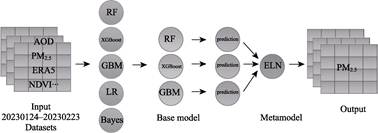
Figure 1  Stacking model architecture diagram

3.2.2 Time-Weighted Calculation of PM_2.5 Exposure Concentration

This study employs a time-weighted method to estimate an individual’s hourly average PM_2.5 exposure. This method comprehensively considers the PM_2.5 concentration encountered at each time point and the duration the individual stays at that point. By accumulating the product of PM_2.5 concentration and duration for these time points and dividing the sum by the individual’s total recorded time during the day, the individual’s hourly average PM_2.5 exposure concentration is obtained. The calculation principle is illustrated in Figure 2. Considering the barrier effect of buildings on air pollution^[14], this study adjusts the estimated individual PM_2.5 exposure concentration based on the method used to acquire trajectory data to determine whether the individual is indoors or outdoors. Data points acquired via GPS signals are classified as outdoor environments, while points recorded using Wi-Fi or Bluetooth are classified as indoor environments. Simultaneously, the PM_2.5 exposure concentration at each stay point is adjusted using an indoor-outdoor exposure correction factor to ensure the accuracy of the assessment results. The time-weighted calculation Equation for individual PM_2.5 exposure concentration is as follows:

                                                              (1)

Whererepresents the individual’s hourly average PM_2.5 exposure (µg/m³),  represents the PM_2.5 concentration (µg/m³) the individual is exposed to while staying in the grid cell,represents the duration of stay (h) in thegrid cell, represents the indoor-outdoor PM_2.5 concentration correction factor. Referring to existing research^[14], this study assumes the coefficient for each indoor/outdoor scenario equals the average value, set to 0.67.  is the total valid recording time (h) for the individual throughout the day. n refers to the total number of grid cells visited during the observation period.

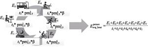
Figure 2  Schematic diagram of hourly average PM_2.5 exposure calculation

To explore differences in PM_2.5 exposure among various groups, this study classified and aggregated the data based on individual characteristic labels and calculated the hourly average PM_2.5 exposure concentration for each group accordingly. This provides an effective quantitative means for assessing and comparing the exposure risks of different groups. The calculation Equation is as follows:

                                                                                 (2)

Whererepresents the group’s average hourly PM_2.5 exposure concentration (µg/m³), andrepresents the number of individuals possessing a specific characteristic. Calculating the hourly average PM_2.5 exposure for groups allows for an effective depiction of exposure risk at the group level on a relatively equitable dimension, thus ensuring the scientific validity of subsequent assessments of PM_2.5 exposure differences among different groups.

3.2.3 Equity Assessment of PM_2.5 Exposure Driven by Group Trajectories

(1) Gini Coefficient Calculation

The Gini Index (GI), a classic statistical tool for measuring inequality, is widely applied in inequality research across various domains such as income distribution, education levels, and health indicators^[15]. Its advantage lies in its ability to comprehensively reflect the degree of inequality in a distribution through a normalized value (ranging from 0 to 1). Additionally, the Gini coefficient is sensitive to changes in the middle range of income or exposure levels. Therefore, this study employs the Gini coefficient to quantify and compare exposure inequality among different cities or groups. The Equation for calculating the Gini coefficient is as follows:

                                                                                                (3)

Whererepresents the difference in PM_2.5 exposure values ​​among individuals (µg/m³), indicating the absolute value of the difference between different individuals within the group.is twice the average PM_2.5 exposure value of all individuals. Here, i and j represent the indices of different individuals within the group, and n is the total sample size within that group. This normalizes the total difference, making the Gini coefficient independent of sample size.

(2) Concentration Index Calculation

Due to computational limitations, the Gini coefficient applies only to unidimensional data and cannot parse the complex relationships among multiple dimensions influencing inequality; For instance, it cannot directly reveal the interaction between income level and PM_2.5 exposure inequality. Therefore, this study employs the Concentration Index (CI)^[16] to explore the relationship between social and spatial characteristics and PM_2.5 exposure inequality. The calculation Equation for the Concentration Index is as follows:

                                                                                         (4)

Where represents the average PM_2.5 exposure level (µg/m³),represents the value of a specific social or spatial characteristic, andrepresents the associated individual’s PM_2.5 exposure concentration (µg/m³). Here, i denotes the rank of the individual after sorting by the social or spatial characteristic value in ascending order, and n is the total sample size. The CI ranges from ‒1 to 1. Taking the correlation between income and PM_2.5 exposure concentration as an example: a CI value close to 0 indicates small exposure differences among groups with different incomes. A CI value less than 0 suggests that low-income groups bear higher exposure burdens, whereas a CI value greater than 0 suggests that high-income groups bear higher exposure burdens.

4 Data Results and Validation

4.1 Dataset Composition

The dataset comprises the following 6 categories of data: (1) hourly 1-km PM_2.5 concentration spatial distribution data of 6 cities from Jan. 24 to Feb. 23, 2023; (2) per capita PM_2.5 exposure concentrations of urban residents derived from dynamic mobile phone trajectory data; (3) hourly average PM_2.5 exposure data of groups in each city classified by social characteristics (age, income and gender) and spatial characteristics (commuting distance); (4) Gini coefficients of PM_2.5 exposure for residents in each city; (5) concentration indices and OLS analysis of PM_2.5 exposure for each population group; (6) hourly average PM_2.5 exposure of residents at the county level. 

4.2 Data Results Analysis

4.2.1 Equity Assessment Results of PM_2.5 Exposure in Each City

The mean hourly PM_2.5 exposure is an intuitive indicator for assessing group exposure levels. As shown in Table 2, Xi’an had the highest mean exposure among the cities at 69.22 µg/m³; conversely, Shenzhen had the lowest mean exposure at just 19.96 µg/m³. The mean exposures for other cities—Chengdu, Wuhan, Shanghai, and Beijing—were 56.36 µg/m³, 50.46 µg/m³, 43.74 µg/m³, and 38.44 µg/m³, respectively. These figures are generally consistent with the annual average monitored PM_2.5 values and their ranking for each city.

The Gini coefficient illustrates the comparison of PM_2.5 exposure inequality across cities. Beijing ranked highest with a Gini coefficient of 0.49, indicating the greatest disparity in PM_2.5 exposure levels among residents within the city. In contrast, Shenzhen, with a Gini coefficient of 0.10, demonstrated a more uniform distribution of PM_2.5 exposure and smaller intra-city disparities.

Table 2  Comparison of urban per capita PM_2.5 exposure concentration and exposure Gini coefficient

4.2.2 Equity Assessment Results of Pollution Exposure for Groups with Different Social Characteristics

Figure 3 presents the summary statistics of hourly average PM_2.5 exposure for groups stratified by income, age, and gender across the six cities. Age group and gender labels originate from the trajectory data provider, covering users aged 22 to 85, grouped in 5-year intervals. Income level uses housing prices in the individual’s area as a proxy variable, classified into 9 levels using a three-class model^[17].

As shown in Table 3, in the income dimension, the CI values for Beijing, Shenzhen, Wuhan, and Chengdu are all greater than 0, indicating that higher PM_2.5 exposure is concentrated among high-income groups in these cities. Conversely, the CI values for Shanghai and Xi’an are less than 0, suggesting that low-income groups bear relatively higher PM_2.5 exposure burdens in these two cities. From the correlation analysis results between different population groups and PM_2.5 exposure, in the age dimension, PM_2.5 exposure among residents in Beijing, Wuhan, Chengdu, and Xi’an declined with age. In contrast, in Shanghai, increasing age was positively correlated with higher PM_2.5 exposure. In the gender dimension, male groups in Beijing and Shanghai experienced higher levels of PM_2.5 exposure compared to female groups, whereas in Chengdu, female exposure levels were higher than male levels.

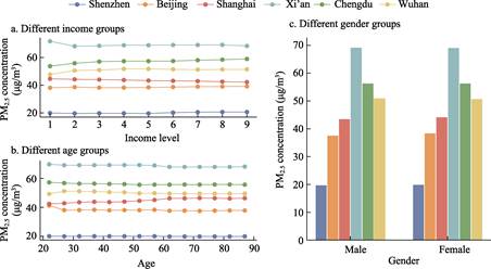
Figure 3  Hourly average PM_2.5 exposure for groups with different social characteristics in each city

Table 3  PM_2.5 exposure concentration index and exposure correlation OLS analysis for groups with different social characteristics in each city

* denotes P<0.1, marginal significance; ** denotes P<0.05, significant; *** denotes P<0.01, highly significant.

4.2.3 Equity Assessment Results of Pollution Exposure for Groups with Different Spatial Characteristics

To explore the differences in PM_2.5 exposure among groups with different spatial characteristics, this study employed a three-class model to categorize residents’ commuting distances, aiming to investigate the relationship between daily commuting distance and PM_2.5 exposure. As shown in Table 4, medium- and long-distance commuters in Beijing and Shanghai experienced higher exposure. Notably, when commuting distance exceeded a certain threshold, exposure levels decreased (Figure 4). In Wuhan, short-distance commuters experienced higher exposure. In Shenzhen, Xi’an, and Chengdu, PM_2.5 exposure was concentrated among medium- and long-distance commuters, although the results were not statistically significant.

Table 4  PM_2.5 exposure concentration index and exposure correlation OLS analysis for groups with different spatial characteristics in each city

* denotes P<0.1, marginal significance; ** denotes P<0.05, significant; *** denotes P<0.01, highly significant.

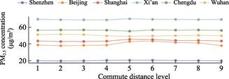
Figure 4  Hourly average PM_2.5 exposure for groups with different commuting distances in each city

Figure 5 depicts the spatial distribution of county-level hourly average PM_2.5 exposure for residents in the six cities. From a spatial distribution perspective, the characteristics of PM_2.5 exposure distribution exhibit significant heterogeneity across cities. In Beijing, populations with high PM_2.5 exposure are mainly distributed in the southeastern and northeastern parts of the city. In Shanghai, residents around the city center have higher PM_2.5 exposure risks, with exposure in some districts being up to 26% higher than in the city center. In Chengdu and Wuhan, residents in the city center experience higher levels of PM_2.5 exposure. Spatial autocorrelation analysis (Moran’s I) shows that resident PM_2.5 exposure in Chengdu and Wuhan exhibits significant positive spatial correlation, with a higher degree of clustering than in other cities, indicating a distinct central agglomeration pattern. Furthermore, the highest PM_2.5 exposure values in Chengdu are located in the southern and southeastern parts of the city. The distribution pattern of PM_2.5 exposure in Xi’an is similar to that in Beijing and Shanghai, primarily concentrated in the suburbs outside the central ring road. Shenzhen’s PM_2.5 exposure distribution exhibits a polycentric pattern.

4.3 Data Validation

The hourly PM_2.5 distribution data used in this study were obtained through predictions from the Stacking ensemble model. The model demonstrated relatively high R² values (ranging from 0.660 to 0.853) and low RMSE values across all cities, with performance significantly superior to traditional single models. It also showed excellent performance across different concentration intervals. Compared with observed daily means, the model’s prediction error rate remained within the 10%–20% range. Compared with semi-annual means, the error rate was only between 0.9% and 10%, indicating good spatiotemporal extrapolation capability and stability. This confirms its reliability and accuracy.

Figure 6 shows the scatter distribution and fitting results of observed versus predicted PM_2.5 concentrations for the six cities. The Stacking model performed robustly across all concentration intervals, with predicted values generally distributed along the 45° diagonal

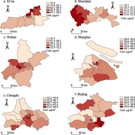
Figure 5  Maps of the county-level hourly average PM_2.5 exposure for residents in each city

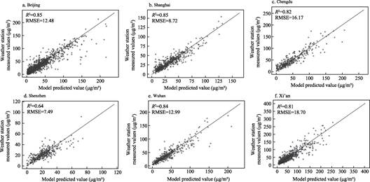
Figure 6  Stacking model fitting results for each city

line, demonstrating good consistency. Some local errors exist, such as slight overestimation in Beijing for the 40–150 μg/m³ range, and similar trends in the high concentration ranges for Shenzhen, Wuhan, as well as Chengdu. This phenomenon may be related to the training data primarily originating from urban centers where PM_2.5 concentrations are generally higher, leading to overestimation at peripheral stations. Overall, the model exhibits high accuracy and stability across different cities.

5 Discussion and Conclusion

This dataset overlays refined trajectory data with high-precision PM_2.5 distribution, employs a time-weighted method to accurately calculate individual and group PM_2.5 exposure concentrations, and subsequently assesses the overall exposure differences among cities, delving into the equity issues of PM_2.5 exposure for groups with different characteristics within cities.

The data results indicate that the time-weighted PM_2.5 exposure concentration estimates are generally consistent with the annual average monitored PM_2.5 values for each city, demonstrating the reliability and stability of the exposure prediction method used in this study. Furthermore, all cities within the study area face a certain degree of inequity in PM_2.5 exposure. Based on the Gini coefficient calculations, inequality is most severe in Beijing, while it is relatively low in Shenzhen, indicating heterogeneity in PM_2.5 exposure disparities across different regions. To elucidate the causes of these differences, this study examined the exposure disparities among groups with different social and spatial characteristics. The results reveal that residents’ PM_2.5 exposure levels are significantly influenced by their social and spatial characteristics, and these influences vary across cities. This phenomenon may be related to the urban structure and industrial layout of the cities. Beijing’s urban structure follows a monocentric ring pattern; residents in the suburbs have relatively fewer job opportunities, leading to longer commuting distances and consequently higher exposure. In Shanghai and Xi’an, heavy polluting industries are located in the suburbs, resulting in higher PM_2.5 concentrations there, indirectly causing suburban residents to bear higher pollution exposure levels. In Wuhan, PM_2.5 pollution concentration is higher in the city center, thus high-income groups in the city center experience higher exposure. In Chengdu, the areas with the highest resident PM_2.5 exposure are in the southern and southeastern parts of the city, which aligns with Chengdu’s polycentric urban layout. Shenzhen’s PM_2.5 exposure distribution is highly consistent with the city’s polycentric structure, showing a polycentric distribution pattern that makes residents’ exposure less influenced by income or commuting distance across different areas.

These results reveal the compound impact of urban spatial layout and industrial distribution on the environmental exposure risks of different population groups and provide a crucial basis for accurately identifying vulnerable groups to PM_2.5 exposure within cities. This offers precise data support for urban PM_2.5 pollution control, facilitates the refinement of environmental measures, and holds significant importance for achieving environmental justice. This dataset covers only 6 cities in China and may not fully reflect the actual situation of PM_2.5 exposure inequality nationwide, although overall, the dataset remains representative to a certain extent. Future research needs to incorporate more influencing factors to further explore the deeper reasons behind the phenomenon of exposure inequality.

Author Contributions

Xia, J. Z. designed the algorithms of dataset. Wu, Z. H. contributed to the data processing and analysis and wrote the data paper. Wu, Z. H. and Ma, Z. F. designed the models and algorithms and performed data validation.

Conflicts of Interest

The authors declare no conflicts of interest.

References

[1]        Chen, H., Kwong, J. C., Copes, R., et al. Exposure to ambient air pollution and the incidence of dementia: a population-based cohort study [J]. Environment International, 2017, 108: 271‒277.

[2]        Guo, Y., Zeng, H., Zheng, R., et al. The association between lung cancer incidence and ambient air pollution in China: a spatiotemporal analysis [J]. Environmental Research, 2016, 144: 60‒65.

[3]        Maji, K. J., Dikshit, A. K., Arora, M., et al. Estimating premature mortality attributable to PM_2.5 exposure and benefit of air pollution control policies in China for 2020 [J]. Science of the Total Environment, 2018, 612: 683‒693.

[4]        Ministry of Environmental Protection, General Administration of Quality Supervision, Inspection and Quarantine. Ambient air quality standard: GB 3095—2012 [S]. 3rd ed. Beijing: China Environmental Science Press, 2012: 3.

[5]        Collins, T. W., Grineski, S. E., Shaker, Y., et al. Communities of color are disproportionately exposed to long-term and short-term PM_2.5 in metropolitan America [J]. Environmental Research, 2022, 214: 114038.

[6]        Ouyang, W., Gao, B., Cheng, H., et al. Exposure inequality assessment for PM_2.5 and the potential association with environmental health in Beijing [J]. Science of the Total Environment, 2018, 635: 769‒778.

[7]        Bravo, M. A., Anthopolos, R., Bell, M. L., et al. Racial isolation and exposure to airborne particulate matter and ozone in understudied US populations: environmental justice applications of downscaled numerical model output [J]. Environment International, 2016, 92: 247‒255.

[8]        Ma, Z. F., Wu, Z. H., Xia, J. Z. 1-km hourly raster dataset of PM_2.5 exposure equality in six cities of China from the trajectory data perspective (Jan. ‒Feb. 2023) [J/DB/OL]. Digital Journal of Global Change Data Repository, 2026. https://doi.org/10.3974/geodb.2026.02.08.V1.

[9]        GCdataPR Editorial Office. GCdataPR data sharing policy [OL]. https://doi.org/10.3974/dp.policy.2014.05 (Updated 2017).

[10]     Chen, Z. Y., Zhang, T. H., Zhang, R., et al. Extreme gradient boosting model to estimate PM_2.5 concentrations with missing-filled satellite data in China [J]. Atmospheric Environment, 2019, 202: 180‒189.

[11]     Danesh Yazdi, M., Kuang, Z., Dimakopoulou, K., et al. Predicting fine particulate matter (PM_2.5) in the Greater London Area: an ensemble approach using machine learning methods [J]. Remote Sensing, 2020, 12(6): 914.

[12]     Sun, J., Gong, J., Zhou, J. Estimating hourly PM_2.5 concentrations in Beijing with satellite aerosol optical depth and a random forest approach [J]. Science of the Total Environment, 2021, 762: 144502.

[13]     Zou, H., Hastie, T. Regularization and variable selection via the elastic net [J]. Journal of the Royal Statistical Society Series B: Statistical Methodology, 2005, 67(2): 301‒320.

[14]     Shao, Z. J. Study on indoor PM_2.5 pollution and its impact on human health [D]. Nanjing: Nanjing University, 2019.

[15]     Jbaily, A., Zhou, X., Liu, J., et al. Air pollution exposure disparities across US population and income groups [J]. Nature, 2022, 601(7892): 228‒233.

[16]     Josa, I., Aguado, A. Measuring unidimensional inequality: practical framework for the choice of an appropriate measure [J]. Social Indicators Research, 2020, 149(2): 541‒570.

[17]     Saunders, P. Social class and stratification [M]. London: Routledge, 2006.