Dataset Development on the Land System and Its Carbon Storage in Sichuan Province, China (2030)

Gao, Y. F.¹  Song, C. Q.²  Huang, J. R.²  Wang, Y. H.²  Ye, S. J.²  Gao, P. C.^1,2*

1. State Key Laboratory of Earth Surface Processes and Disaster Risk Reduction, Beijing Normal University, Beijing 100875, China;

2. Center for Geodata and Analysis, Faculty of Geography, Beijing Normal University, Beijing 100875, China

Abstract: This study employs the CLUMondo model to predict changes in Sichuan Province??s land systems from 2020 to 2030 and estimates the region??s carbon storage for 2030 while integrating land-use intensity under ecological-economic trade-off scenarios. The predicted land system data and carbon storage estimates form the ??Predicting land system and carbon storage dataset of Sichuan Province of China in 2030??. The dataset includes: (1) raster data of land system in Sichuan Province for the years 2010, 2020, and predicted raster data of land system data in 2030 under 9 scenarios; (2) estimated carbon storage of Sichuan Province in 2030 under 9 scenarios; (3) carbon density. The spatial resolution of the land system raster data is 1 km. The dataset is archived in .tif and .xlsx data formats, and consists of 18 data files with a data size of 51.4 MB (Compressed into one file with 1.84 MB).

Keywords: land system data; CLUMondo; carbon storage assessment; Sichuan Province

DOI: https://doi.org/10.3974/geodp.2025.01.09

Dataset Availability Statement:

The dataset supporting this paper was published and is accessible through the Digital Journal of Global Change Data Repository at: https://doi.org/10.3974/geodb.2024.11.04.V1.

1 Introduction

Controlling the continuous rise in global temperatures has become a core objective of climate pledges. In 2015, at the 21st Conference of the Parties (COP21) held in Paris, it was proposed to hold the global average temperature increase to well below 2 ??C above preindustrial levels and pursue efforts to limit the temperature increase to 1.5 ??C^[1]. In 2021, at the 26th Conference of the Parties (COP26) in Glasgow, 154 parties updated or submitted new climate pledges and reaffirmed the 1.5 ??C climate goal^[2]. To mitigate climate change, China has set the goal of achieving carbon neutrality by 2060^[3], making it a crucial development priority and an essential objective^[4]. The primary driver of global temperature rise is the increasing carbon dioxide emissions from human activities. The main sources of increasing carbon dioxide emissions from human activities are fossil fuel combustion and land-use changes. Since the Industrial Revolution, carbon emissions from land-use changes have accounted for approximately one-third of the total emissions from human activities, making them a significant driver of global temperature rise^[5].

Sichuan Province is a critical region in China??s path to carbon neutrality. Sichuan Province is abundant in forest resources, with forest areas covering approximately 40% of its total land area^[6]. Notably, forests are the largest ??carbon sinks?? in terrestrial ecosystems and play a key role in absorbing carbon dioxide from the atmosphere^[7]. At the same time, future land demands in Sichuan Province show clear ecological-economic trade-offs. For example, the 14th Five-Year Plan for Economic and Social Development and Vision for 2035 of Sichuan Province outlined that by 2035, Sichuan Province needs to achieve ??significant economic growth??. However, it is difficult for any land type to achieve high ecological and economic benefits simultaneously.

Given the above background, there is a need for future land data and carbon storage estimates to provide data support for balancing economic and ecological benefits in land management for Sichuan Province. This study uses the CLUMondo model, which incorporates ecological-economic trade-offs and land-use intensity, to predict land system changes for Sichuan Province in 2030 and estimate its carbon storage.

2 Metadata of the Dataset

The name, authors, geographic region, data years, spatial resolution, dataset composition, data publication and sharing platform, and data sharing policies for the Predicting land system and carbon storage dataset of Sichuan Province of China in 2030^[8], are provided in Table 1.

3 Methods   

3.1 Data Sources

The dataset materials used in this study include land cover data, driving factor data, data for calculating supply capacity, and carbon density spatial distribution data. The land cover data are used to generate the land system data. Driving factor data are used as input to calculate location suitability, which determines the likelihood of changing each land type driven by social, natural, and economic factors. Supply capacity represents the ability of each land type to provide different land system services. Carbon density spatial distribution data are used to calculate the carbon density coefficients for each land system type. The detailed data are shown in Table 2.

3.2 Algorithm

3.2.1 Land System Modeling Based on Land-Use Intensity

Land system data are generated by reclassifying land use/land cover types based on datasets that reflect the natural state of the surface, socioeconomic factors, or the density of land use/land cover types. Land system data were first proposed and utilized by Verburg^[15] and have since been widely applied in land change modeling^[16,17]. Compared with land cover/use data, land system data reflect not only land use types but also the density or social,

Table 1  Metadata summary of Predicting land system and carbon storage dataset of Sichuan Province of China in 2030

Table 2  Data sources

(To be continued on the next page)

(Continued)

(To be continued on the next page)

(Continued)

natural, and economic factors.

In this study, Globeland30 data^[10,11] were used to generate land system data in 2010 and 2020 at a 1 km resolution using upscaling methods^[16,18]. The 2010 and 2020 land system data can reflect the local density of the dominant type. The process for generating the land system data is shown in Figure 1. Specifically, the process of generating land system data consists of three steps. First, the size of the sliding window was determined. Next, for each sliding window, the land cover type with the largest area was identified as the dominant type. This dominant type determines the system type for the upscaled pixel. For example, in a sliding window, if the land cover type with the largest area was cropland, the upscaled pixel would be classified as a ??cropland system??. Third, the density type for the upscaled pixel was determined based on natural break thresholds. The method for calculating natural break thresholds is to slide the global Globeland30 data using a 33??33 sliding window. For each sliding window, the proportion of the dominant land cover type was calculated. All proportions of each land cover type were then used to calculate the natural break thresholds.

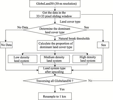
Figure 1  Flowchart of the land system data development

3.2.2 Land System Services and Scenario Design Considering Ecological‒Economic Trade-offs

The scenario design includes the setup of land system services and calculating their values in 2030. This study sets 2 land system services, namely Gross Domestic Product (GDP) and Gross Ecosystem Product (GEP). The GDP represents economic benefits, whereas the GEP represents ecological benefits. The total GDP for 2020 was obtained from statistical yearbooks, and the total GEP for 2020 was derived by calculating the sum of GEP grid data within Sichuan Province. The GEP grid data are categorized into 4 major services, namely provisioning, regulating, supporting, and cultural services^[19]. To emphasize ecological functions, the calculation of GEP in this study only focuses on regulating, supporting, and cultural services. Through combinations of 3 different levels of annual GDP growth rates and 3 different levels of annual GEP growth rates, 9 scenarios were designed in the study. The GDP growth rates are set at 3.00%, 4.00%, and 5.00%, whereas the GEP growth rates are set at 0.05%, 0.50%, and 1.00%. The total GDP and GEP for Sichuan Province in 2030 under each scenario are shown in Table 3.

Table 3  Total GDP and GEP of Sichuan Province in 2030 under nine scenarios

3.2.3 Land System Change Simulation Based on the CLUMondo Model

The original version of the CLUMondo model was developed by van Asselen and Verburg in 2012^[15]. The CLUMondo model has been widely used in global and regional land change simulations^[20?C23]. The principle of the CLUMondo model is that land types change iteratively through land type conversion rules to respond to changes in all land system services^[18,24]. The core characteristic of the CLUMondo model is its ability to establish the many-to-many relationships between land system types and land system services^[24]. Specifically, each land type provides multiple services, and each service can be met by multiple land types. The basic principle of the CLUMondo model is illustrated in Figure 2.

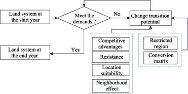
Figure 2  Principles of the CLUMondo model

To simulate land system changes using CLUMondo, it is necessary to calculate location suitability, supply capacity, conversion order, resistance, and conversion matrix. The location suitability reflects the likelihood of each land type changing into any land type driven by various natural, social, and economic factors. The resistance indicates the difficulties for one land type to be converted into others. The conversion matrix indicates restrictions on the changes that are not allowed between land types. The calculation methods are as follows.

(1) Location suitability

Before calculating location suitability, this study normalized the driving factors and removed those with high correlations. The correlation between the driving factors was assessed using Spearman??s correlation coefficient, as it does not require the variables to follow a normal distribution. In this study, the rule for removing driving factors with high correlations consists of 3 steps. First, Spearman??s correlation coefficients between all pairs of driving factors were calculated. Second, driving factors with a coefficient greater than 0.8 were identified. Third, for these pairs, the sum of their correlation coefficients with all other driving factors was calculated, and the driving factor with the larger sum was removed.

In the CLUMondo model, the calculation of location suitability is performed through logistic regression, as shown in Equation 1. SPSS software was used in this study to conduct logistic regression for each land system. The sample proportion selected for regression was 100%, and the regression method used was ??Forward: Conditional??.

                                          (1)

whererepresent the values of the driving factors at the pixel, are the coefficients of the driving factors, andis the constant term.  represents the local suitability to change to land type j at the pixel. The value ofranges from, with higher values indicating greater suitability.

(2) Supply capacity

Supply capacity represents the quantity of land system services that each land type can serve. In this study, the land system services consist of GDP and GEP. The supply capacities were calculated by overlaying the 2020 land system data with the 2020 GDP raster data and GEP raster data. The overlay analysis calculates the average GDP and GEP for each land system type. The average GDP and GEP for each land system type serve as the supply capacity. For GDP, due to discrepancies between the total amount obtained from raster data and the statistical yearbook for Sichuan Province, this study calibrated the raster data??s total GDP by multiplying it with a coefficient. The calculation method for the coefficient is shown in Equation 2. The supply capacity of each land system service for Sichuan Province, as calculated in this study, is presented in Table 4.

                                                                                                       (2)

whereis the coefficient,is the total GDP for Sichuan Province obtained from the GDP raster data, andis the total GDP for Sichuan Province as reported in the statistical yearbook.

(3) Conversion order

The conversion order reflects the capacity of each land system type to meet each land system service. The conversion order values are represented by ???C1?? and nonnegative integers. A value of ???C1?? indicates that the land system is unable to serve the land system service. Nonnegative integers represent the strength of the supply capacity, with higher values indicating greater capacity to serve the land system service. In this study, the conversion orders are assigned based on the supply capacity of land systems^[18]. Specifically, the supply capacity values of the land systems are ranked. For land systems that cannot provide service, the conversion order value is set to ???C1,?? while for the remaining land system types, it is assigned values starting from ??0?? based on supply capacity. If there is the same supply capacity in multiple land systems, they are assigned the same conversion order value. Additionally, to ensure more reasonable simulation results, this study sets the conversion order for low-density, medium-density, and high-density water bodies for GEP to ??0?? to reduce large-scale conversion from other land types to water bodies. The conversion order settings used in this study are shown in Table 4.

Table 4  Supply capacity and conversion order statistics

(To be continued on the next page)

(Continued)

(4) Resistance

The resistances in this study are calculated based on historical changes in land systems. The easier it is for a land system type to change into other land system types during a specific historical period, the smaller its resistance. Conversely, the more difficult the changes, the larger the resistance. According to the meaning of resistances, the calculation method of resistances is provided in Equation 3. The results of the resistances are shown in Table 5.

Table 5  Resistance for each land type

                                                                                                (3)

whererepresents the resistance of land type.anddenote 2 historical years, with.represents the number of pixels that remain unchanged as land typein both yearsand, whereas represents the number of pixels classified as land typein year.

(5) Conversion matrix

The conversion matrix is also determined based on historical changes in land systems. If land system typehas been changed into land system typein historical changes, then the conversion from land typeto land typeis allowed.

3.2.4 Estimation of Carbon Storage Based on the Carbon Density of Land System Types

The basic principle for estimating carbon storage is to multiply the area of each land system type by its corresponding carbon density coefficient and then sum the results. The key step is to calculate the carbon density coefficient for each land system type^[25]. When calculating carbon storage (), four carbon pools are considered, namely aboveground carbon storage, belowground carbon storage, soil carbon storage, and dead biomass organic carbon storage^[26]. Due to the challenges in obtaining data on dead biomass organic carbon storage, this study follows previous research by excluding dead biomass organic carbon storage from the calculation. The calculation of carbon storage in this study is shown in Equation 4. The carbon density coefficient for each land system type is obtained by overlaying land system data with spatial distribution data of carbon density. The carbon density coefficient of each land system type is the average carbon density corresponding to that land system type, with the calculation methods shown in Equations 5 to 7. The calculation results for the carbon density coefficients are presented in the Predicting land system and carbon storage dataset of Sichuan Province of China in 2030^[8].

                                                                            (4)

                                                                                                (5)

                                                                                                 (6)

                                                                                                    (7)

whererepresents the area of the-th land system type (ha),represents the aboveground biomass carbon density of the-th land system type (MgC/ha),represents the belowground biomass carbon density of the-th land system type (MgC/ha), andrepresents the soil carbon density of the -th land system type (MgC/ha). , , and  denote the aboveground biomass carbon density, belowground biomass carbon density, and soil carbon density, respectively, of the -th pixel of the -th land system type.  is the area of the -th pixel of the -th land system type.

3.3 Technical Workflow

The technical workflow of this study is shown in Figure 3. The workflow consists of 5 parts. First, land system data for Sichuan Province for 2010 and 2020 are created. Second, parameters, including resistance, the conversion matrix, location suitability, supply capacity, and the conversion order, are calculated. Third, scenarios are set. This study uses GDP to reflect economic benefits and GEP to reflect ecological benefits. By setting different annual growth rates, the GDP and GEP for Sichuan Province in 2030 are obtained. Fourth, land system changes in Sichuan Province from 2020 to 2030 are predicted. Fifth, the carbon density coefficients of land system types are calculated, and carbon storage in 2030 is predicted.

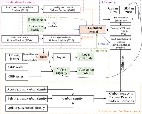
Figure 3  Workflow of the dataset development

4 Data Results and Validation

4.1 Dataset Composition

The composition of the dataset is shown in Table 6. The dataset consists of 2 parts, namely land system data and carbon storage data. The land system data are available for the years 2010, 2020, and 2030 in .tif format with a spatial resolution of 1 km. The carbon storage data are available for the years 2020 and 2030, stored in .xlsx format.

Table 6  Dataset composition

4.2 Data Results

4.2.1 Land System Prediction Results

This study developed land system maps in Sichuan Province for 2010 and 2020 and predicted land system changes from 2020 to 2030 using the CLUMondo model. The land system maps for 2010 and 2020 are shown in Figure 4, while the land system maps for 2030 under 9 scenarios are shown in Figure 5. As observed in Figure 5, with GDP growth, the southeastern region of Sichuan Province will experience increased cropland density and urban expansion due to cropland encroachment. The higher the annual GDP growth rate, the greater the expansion of urban agglomerations centered around Chengdu. With GEP growth, the northwestern region of Sichuan Province will experience further increases in the density and expansion of forests and grasslands, promoting wetland conservation and restoration in the northern part of the province.

Figure 4  Land system maps in 2010 and 2020

4.2.2 Carbon Storage Prediction Results

The predicted carbon storage results in Sichuan Province under nine scenarios are detailed in the Predicting land system and carbon storage dataset of Sichuan Province of China in 2030^[8]. The results indicate that carbon storage in 2030 under the S3 scenario shows the largest increase among all scenarios. Compared to 2020, the carbon storage under the S3 scenario increases by 2.89%. In terms of carbon storage components, the increase comes from aboveground biomass carbon storage and belowground biomass carbon storage, which increase by 13.67% and 7.37%, respectively. From the perspective of land types, the increase in carbon storage is attributed primarily to the expansion of high-density forests, which originates mainly from the conversion of medium- and high-density grasslands as well as low- and medium-density forests. In contrast, the carbon storage under the S7 scenario in 2030 shows the largest decrease among all scenarios. Compared to 2020, carbon storage will decrease by 3.23%. The decrease is mainly due to a decrease in belowground biomass carbon storage and soil carbon storage, which will decrease by 2.29% and 4.83%, respectively.

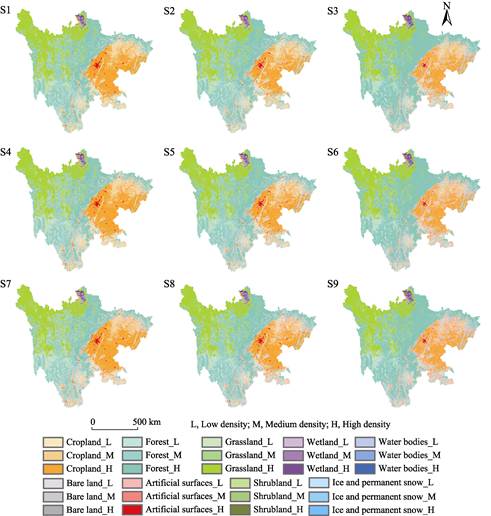
Figure 5  Land system maps for 2030 under all scenarios

4.3 Data Validation

The basic assumption for data validation in this study is that if the CLUMondo model can effectively simulate historical land system changes, it can also reliably predict future land  system changes. Based on this assumption, the study simulated land system changes in Sichuan Province from 2010 to 2020. Then the simulated land system data in 2020 is compared with the actual land system data in 2020.

This study uses the Kappa coefficient and figure of merit (FoM) to evaluate the accuracy of the land change simulations. Both the Kappa coefficient and FoM assess model accuracy from different perspectives. The Kappa coefficient is used to evaluate the similarity between the simulated results and the actual land system map^[27], whereas the FoM calculates the proportion of correctly simulated pixels compared with the total number of correctly changed pixels to assess the accuracy of the changes^[28]. The calculation method for the Kappa coefficient is shown in Equation 8. The value of the Kappa coefficient ranges from , with a higher value indicating better simulation accuracy. The calculation method for FoM is shown in Equation 9. The value of FoM ranges from , with a higher value indicating better simulation accuracy.

                                                                                                        (8)

                                                              (9)

where is the overall accuracy, which represents the proportion of correctly simulated pixels for land types;represents the proportion of correctly simulated pixels randomly. refers to the number of pixels that actually changed in the land change simulation and were correctly predicted in the simulation;refers to the number of pixels that changed in the actual land change process but were not predicted to change in the simulation. False alarm refers to the number of pixels that did not change in reality but were predicted to change in the simulation.refers to the number of pixels that changed in reality but were incorrectly predicted to change in the simulation.

The Kappa coefficient and FoM results both demonstrate the excellent performance of the land change simulation in this study. As shown in Table 7, the Kappa coefficient reached 83.4% for the 27 land types, and after the 27 land types were merged into 9 categories, the Kappa coefficient was 89.0%. Although the FoM value was relatively low for the 27 land types, it increased by 109.0% after the land types were merged into 9 categories. Compared with similar studies, the land change simulation accuracy in this study is relatively high. For example, in reference^[29], the FoM for 5 land types was approximately 7.0%; in reference^[30], the FoM reached approximately 50.0%, but this study considered only 2 land types, and the FoM calculation did not account for Miss, which caused the FoM value to be overstated.

5 Discussion and Conclusion

This study uses the CLUMondo model to predict land system changes in Sichuan Province from 2020 to 2030, based on a balance between ecological and economic benefits and land-use intensity. Additionally, the carbon storage of Sichuan Province in 2030 was estimated based on the predicted land system data. Compared with similar studies, the land system data predicted in this study have a higher thematic resolution, providing a more detailed depiction of future land changes in Sichuan Province. Furthermore, through overlay analysis, the carbon density coefficients for land system types were calculated more accurately, leading to a more precise prediction of future carbon storage changes in Sichuan Province.

The data produced in this study have 2 significant implications. First, the land system data and carbon storage estimation data predicted in this study can provide data support for achieving coordinated ecological-economic development in Sichuan Province in land management. Second, the data produced can serve as data support for multiple scientific fields. For example, predicted land system data can provide basic data support for studies on biodiversity assessment, flood risk analysis, water cycling, and other research areas.

Author Contributions

Gao, P. C. and Song, C. Q. contributed to the overall design of the dataset development; Gao Y. F. collected and processed and performed the data validation, and wrote the data paper; Wang, Y. H., Ye, S. J. and Huang, J. R. supervised the writing of the paper.

Conflicts of Interest

The authors declare no conflicts of interest.

References

[1]        Schleussner, C. F., Rogelj, J., Schaeffer, M., et al. Science and policy characteristics of the Paris Agreement temperature goal [J]. Nature Climate Change, 2016, 6(9): 827‒835. DOI: 10.1038/nclimate3096.

[2]        Meinshausen, M., Lewis, J., Mcglade, C., et al. Realization of Paris Agreement pledges may limit warming just below 2 ??C [J]. Nature, 2022, 604(7905): 304‒309. DOI: 10.1038/s41586-022-04553-z.

[3]        Gao, P. C., Song, C. Q. Review: Climate Economics and the Future of Humanity [J]. Economic Geography, 2021, 41(10): 41.

[4]        Mallapaty, S. How China could be carbon neutral by mid-century [J]. Nature, 2020, 586(7830): 482‒484. DOI: 10.1038/d41586-020-02927-9

[5]        Brovkin, V., Sitch, S., Von Bloh, W., et al. Role of land cover changes for atmospheric CO₂ increase and climate change during the last 150 years [J]. Global Change Biology, 2004, 10(8): 1253‒1266. DOI: 10.1111/j.1365-2486.2004.00812.x.

[6]        Hu, J. X., Huang, F., Tie, L. H., et al. Economic value dynamics of carbon sequestration in forest vegetation of Sichuan Province [J]. Acta Ecologica Sinica, 2019, 39(1): 158‒163. DOI: 10.5846/stxb201809292123.

[7]        Huang, C. D., Zhang, J., Yang, W. Q., et al. Spatial differentiation characteristics of forest vegetation carbon stock in Sichuan Province [J]. Acta Ecologica Sinica, 2009, 29(9): 5115‒5121.

[8]        Gao, Y. F., Song, C. Q., Huang, J. R., et al. Predicting land system and carbon storage dataset of Sichuan Province of China in 2030 [J/DB/OL]. Digital Journal of Global Change Data Repository, 2024. https://doi.org/10.3974/geodb.2024.11.04.V1.

[9]        GCdataPR Editorial Office. GCdataPR data sharing policy [OL]. https://doi.org/10.3974/dp.policy.2014.05 (Updated 2017).

[10]     Chen, J., Ban, Y. F., Li, S. N. China: open access to Earth land-cover map [J]. Nature, 2014, 514(7523): 434‒434. DOI: 10.1038/514434c.

[11]     Chen, J., Chen, J., Liao, A. P., et al. Global land cover mapping at 30 m resolution: a POK-based operational approach [J]. ISPRS Journal of Photogrammetry and Remote Sensing, 2015, 103: 7‒27. DOI: 10.1016/j.isprsjprs.2014.09.002.

[12]     National Bureau of Statistics of China. China Statistical Yearbook [M]. Beijing: China Statistics Press, 2020.

[13]     Poggio, L., De Sousa, L. M., Batjes, N. H., et al. SoilGrids 2.0: producing soil information for the globe with quantified spatial uncertainty [J]. Soil, 2021, 7(1): 217‒240. DOI: 10.5194/soil-7-217-2021.

[14]     Spawn, S. A., Sullivan, C. C., Lark, T. J., et al. Harmonized global maps of above and belowground biomass carbon density in the year 2010 [J]. Scientific Data, 2020, 7(1): 1‒22. DOI: 10.1038/s41597-020-0444-4.

[15]     van Asselen, S., Verburg, P. H. A land system representation for global assessments and land-use modeling [J]. Global Change Biology, 2012, 18(10): 3125‒3148. DOI: 10.1111/j.1365-2486.2012.02759.x.

[16]     Gao, P. C., Gao, Y. F., Ou, Y., et al. Fulfilling global climate pledges can lead to major increase in forest land on Tibetan Plateau [J]. iScience, 2023, 26(4): 106364. DOI: 10.1016/j.isci.2023.106364.

[17]     Jin, X. L., Jiang, P. H., Ma, D. X., et al. Land system evolution of Qinghai-Tibetan Plateau under various development strategies [J]. Applied Geography, 2019, 104: 1‒9. DOI: 10.1016/j.apgeog.2019.01.007.

[18]     Gao, P. C., Gao, Y. F., Zhang, X. D., et al. CLUMondo-BNU for simulating land system changes based on many-to-many demand?Csupply relationships with adaptive conversion orders [J]. Scientific Reports, 2023, 13(1): 5559. DOI: 10.1038/s41598-023-31001-3.

[19]     Xie, G. D., Zhang, C. X., Zhang, L. M., et al. Improvement of the evaluation method for ecosystem service value based on per unit area [J]. Journal of Natural Resources, 2015, 30(8): 1243‒1254. DOI: 10.11849/zrzyxb.2015.08.001.

[20]     van Asselen, S., Verburg, P. H. Land cover change or land-use intensification: simulating land system change with a global-scale land change model [J]. Global Change Biology, 2013, 19(12): 3648‒3667. DOI: 10.1111/gcb.12331.

[21]     Domingo, D., Palka, G., Hersperger, A. M. Effect of zoning plans on urban land-use change: a multi-scenario simulation for supporting sustainable urban growth [J]. Sustainable Cities and Society, 2021, 69: 102833. DOI: 10.1016/j.scs.2021.102833.

[22]     Malek, Ž., Verburg, P. H., Geijzendorffer, I. R., et al. Global change effects on land management in the Mediterranean region [J]. Global Environmental Change, 2018, 50: 238‒254. DOI: 10.1016/j.gloenvcha. 2018.04.007.

[23]     Wang, Y., van Vliet, J., Pu, L. J., et al. Modeling different urban change trajectories and their trade-offs with food production in Jiangsu Province, China [J]. Computers, Environment and Urban Systems, 2019, 77: 101355. DOI: 10.1016/j.compenvurbsys.2019.101355.

[24]     van Vliet, J., Verburg, P. H. A short presentation of CLUMondo [M]//Mar??a Teresa Camacho Olmedo, Paegelow, M., Mas, J. F., et al. Geomatic Approaches for Modeling Land Change Scenarios. Cham: Springer International Publishing, 2018: 485‒492.

[25]     Gao, Y. F., Song, C. Q., Wang, Y. H., et al. Carbon storage prediction of terrestrial ecosystems and hotspot analysis in Sichuan Province by considering land use intensity and eco-economic trade-offs [J]. Acta Ecologica Sinica, 2024, 44(9): 1‒12. DOI: 10.20103/j.stxb.202211113250.

[26]     Shao, Z., Chen, R., Zhao, J., et al. Spatio-temporal evolution and prediction of carbon storage in Beijing??s ecosystem based on FLUS and InVEST models [J]. Acta Ecologica Sinica, 2022, 42(23): 1‒14. DOI: 10.5846/stxb202201100094.

[27]     van Vliet, J., Bregt, A. K., Hagen-Zanker, A. Revisiting Kappa to account for change in the accuracy assessment of land-use change models [J]. Ecological Modelling, 2011, 222(8): 1367‒1375. DOI: 10.1016/j.ecolmodel.2011.01.017.

[28]     Zhang, T. Y., Cheng, C. X., Wu, X. D. Mapping the spatial heterogeneity of global land use and land cover from 2020 to 2100 at a 1 km resolution [J]. Scientific Data, 2023, 10(1): 748. DOI: 10.1038/s41597-023-02637-7.

[29]     Zhang, J. D., Mei, Z. X., Lv, J. H., et al. Simulating multiple land use scenarios based on the FLUS Model considering spatial autocorrelation [J]. Journal of Geo-information Science, 2020, 22(3): 531‒542. DOI: 10.12082/dqxxkx.2020.190359.

[30]     Wang, H., Zeng, Y. N. Urban expansion model based on extreme learning machine [J]. Acta Geodaetica et Cartographica Sinica, 2018, 47(12): 1680‒1690. DOI: 10.11947/j.AGCS.2018.20170586.